18.657: Mathematics of Machine Learning
Lecturer: Philippe Rigollet
Scribe: Kevin Li
Lecture 11
Oct. 14, 2015
2. CONVEX OPTIMIZATION FOR MACHINE LEARNING
In this lecture, we will cover the basics of convex optimization as it applies to machine
learning. There is much more to this topic than will be covered in this class so you may be
interested in the following books.
Convex Optimization by Boyd and Vandenberghe
Lecture notes on Convex Optimization by Nesterov
Convex Optimization: Algorithms and Complexity by Bubeck
Online Convex Optimization by Hazan
The last two are drafts and can be obtained online.
2.1 Convex Problems
A convex problem is an optimization problem of the form min f (x) where f and C are
x∈C
convex. First, we will debunk the idea that convex problems are easy by showing that
virtually all optimization problems can be written as a convex problem. We can rewrite an
optimization problem as follows.
min f (x)
X ∈X
⇔
,
min
t≥f (x),x∈X
t
⇔
,
min
t
(x,t)∈epi(f )
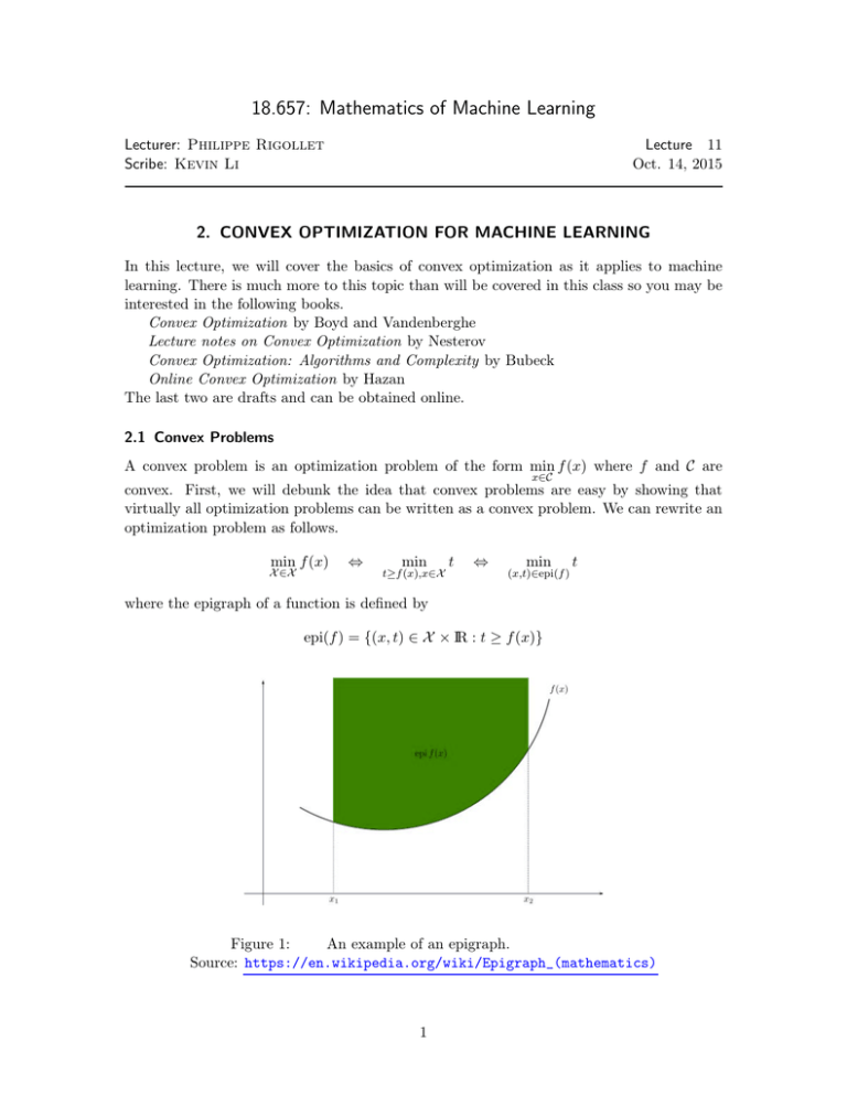
where the epigraph of a function is defined by
∈ X × IR : t ≥ f (x)g}
epi(f ) = {f(x, t) 2
Figure 1:
An example of an epigraph.
Source: https://en.wikipedia.org/wiki/Epigraph_(mathematics)
1
Now we observe that for linear functions,
min c> x =
x∈D
min
c> x
x∈conv(D)
where the convex hull is defined
conv(D) = {fy : ∃
9N ∈
2 Z+ , x1 , . . . , xN ∈
2 D, αi ≥ 0,
N
X
αi = 1, y =
i=1
N
X
αi xi }g
i=1
To prove this, we know that the left side is a least as big as the right side since D ⊂ conv(D).
For the other direction, we have
min
x∈conv(D)
>
c x = min
N
= min
N
≥ min
N
>
min
min c
x1 ,...,xN ∈D α1 ,...,αN
min
min
x1 ,...,xN ∈D α1 ,...,αN
min
min
x1 ,...,xN ∈D α1 ,...,αN
N
X
αi xi
i=1
N
X
i=1
N
X
αi c> xi ≥ min c> x
x∈D
αi min c> x
x∈D
i=1
= min c> x
x∈D
Therefore we have
min f (x) ⇔
,
x∈X
min
t
(x,t)∈conv(epi(f ))
which is a convex problem.
Why do we want convexity? As we will show, convexity allows us to infer global information from local information. First, we must define the notion of subgradient.
→ IR. A vector g ∈
Definition (Subgradient): Let C ⊂ IRd , f : C !
2 IRd is called a
subgradient of f at x ∈
2 C if
f (x) − f (y) ≤ g > (x − y)
∀
8y ∈
2C.
The set of such vectors g is denoted by ∂f (x).
Subgradients essentially correspond to gradients but unlike gradients, they always exist for convex functions, even when they are not differentiable as illustrated by the next
theorem.
→ IR is convex, then for all x, ∂f (x) 6= ∅;. In addition, if f is
Theorem: If f : C !
}
differentiable at x, then ∂f (x) = {∇
frf (x)g.
Proof. Omitted. Requires separating hyperplanes for convex sets.
2
Theorem: Let f, C be convex. If x is a local minimum of f on C, then it is also global
minimum. Furthermore this happens if and only if 0 2
∈ ∂f (x).
Proof. 0 2
2 C. This is clearly equivalent to
∈ ∂f (x) if and only if f (x) − f (y) ≤ 0 for all y ∈
x being a global minimizer.
Next assume
∈ C there exists ε small enough such
x is a local minimum. Then for all y 2
⇒ f (x) ≤ f (y) for all y 2
∈ C.
that f (x) ≤ f (1 − ε)x + εy ≤ (1 − ε)f (x) + εf (y) =)
Not only do we know that local minimums are global minimums, looking at the subgradient also tells us where the minimum can be. If g > (x − y) < 0 then f (x) < f (y). This
means f (y) cannot possibly be a minimum so we can narrow our search to ys such that
g > (x − y). In one dimension, this corresponds to the half line fy
{ 2
∈ IR : y ≤ xg} if g > 0 and
the half line fy
{ 2
∈ IR : y ≥ xg} if g < 0 . This concept leads to the idea of gradient descent.
2.2 Gradient Descent
y ≈ x and f differentiable the first order Taylor expansion of f at x yields f (y) ≈ f (x) +
g > (y − x). This means that
min f (x + εµ̂) ≈ min f (x) + g > (εµ̂)
|µ̂|2 =1
which is minimized at µ̂ = − |g|g 2 . Therefore to minimizes the linear approximation of f at
x, one should move in direction opposite to the gradient.
Gradient descent is an algorithm that produces a sequence of points fx
{ j }gj≥1 such that
(hopefully) f (xj+1 ) < f (xj ).
Figure 2: Example where the subgradient of x1 is a singleton and and the subgradient of
x2 contains multiple elements.
Source: https://optimization.mccormick.northwestern.edu/index.php/
Subgradient_optimization
3
Algorithm 1 Gradient Descent algorithm
Input: x1 2
∈ C, positive sequence fη
{ s }gs≥1
for s = 1 to k − 1 do
xs+1 = xs − ηs gs , gs ∈
2 ∂f (xs )
end for
k
1X
return Either x̄ =
xs or x◦ 2
∈ argmin f (x)
k
x∈{x1 ,...,xk }
s=1
Theorem: Let f be a convex L-Lipschitz function on IRd such that x∗ 2
∈ argminIRd f (x)
R
∗
√
exists. Assume that jx
| 1 − x |j2 ≤ R. Then if ηs = η = L k for all s ≥ 1, then
f(
and
k
1X
LR
√
xs ) − f (x∗ ) ≤ p
k
k
s=1
LR
√
min f (xs ) − f (x∗ ) ≤ p
k
1≤s≤k
Proof. Using the fact that gs = η1 (xs+1 − xs ) and the equality 2a> b = kak
k k2 + kbk
k k2 − ka
k − bkk2 ,
1
f (xs ) − f (x∗ ) ≤ gs> (xs − x∗ ) = (xs − xs+1 )> (xs − x∗ )
η
i
1h
=
kxs − xs+1 k2 + kxs − x∗ k2 − kxs+1 − x∗ k2
2η
η
1
2
= kg
)
k s k2 + (δs2 − δs+1
2
2η
where we have defined δs = kx
k s − x∗ kk. Using the Lipschitz condition
f (xs ) − f (x∗ ) ≤
η 2
1
2
L + (δs2 − δs+1
)
2
2η
Taking the average from 1, to k we get
k
1X
η
1
η
1 2 η 2
R2
f (xs ) − f (x∗ ) ≤ L2 +
(δ12 − δs2+1 ) ≤ L2 +
δ1 ≤ L +
k
2
2k η
2
2kη
2
2kη
s=1
Taking η =
R
√
L k
to minimize the expression, we obtain
k
1X
LR
√
f (xs ) − f (x∗ ) ≤ p
k
k
s=1
Noticing that the left-hand side of the inequality is larger than both f (
k
P
s=1
xs ) − f (x∗ ) by
Jensen’s inequality and min f (xs ) − f (x∗ ) respectively, completes the proof.
1≤s≤k
4
One flaw with this theorem is that the step size depends on k. We would rather have
step sizes ηs that does not depend on k so the inequalities hold for all k. With the new step
sizes,
k
X
∗
ηs [f (xs ) − f (x )] ≤
s=1
k
X
η2
s=1
k
k
s=1
s=1
X L R2
1X 2
2
L +
(δs − δs+1
)≤
ηs2
+
2
2
2
2
s
2
P
After dividing byP ks=1 ηs , we would like the right-hand side to approach 0. For this to
2
P
happen we need P ηηss →
! 0 and
ηs →
!∞
1. One candidate for the step size is ηs = √Gs since
k
k
√
p
P
P
then
ηs2 ≤ c1 G2 log(k) and
ηs ≥ c2 G k. So we get
s=1
s=1
k
X
s=1
ηs
k
−1 X
ηs [f (xs ) − f (x∗ )] ≤
s=1
c1 GL log k
R2
√
√
p
p
+
2c2 k
2c2 G k
q
Choosing G appropriately, the right-hand side approaches 0 at the rate of LR logk k . Notice
√
p
that we get an extra factor of log k. However, if we look at the sum from k/2 to k instead
k
k
√
p
P
P
ηs2 ≤ c01 G2 and
ηs ≥ c02 G k. Now we have
of 1 to k,
s= k2
s=1
min f (xs ) − f (x∗ ) ≤ min f (xs ) − f (x∗ ) ≤
1≤s≤k
k
≤s≤k
2
k
X
s= k2
ηs
k
−1 X
cLR
p
ηs [f (xs ) − f (x∗ )] ≤ √
k
k
s= 2
which is the same rate as in the theorem and the step sizes are independent of k.
Important Remark: Note this rate only holds if we can ensure that |jxk/2 − x∗ |j2 ≤ R
since we have replaced x1 by xk/2 in the telescoping sum. In general, this is not true for
gradient descent, but it will be true for projected gradient descent in the next lecture.
One final remark is that the dimension d does not appear anywhere in the proof. However, the dimension does have an effect because for larger dimensions, the conditions f is
L-Lipschitz and |jx1 − x∗ j|2 ≤ R are stronger conditions in higher dimensions.
5
MIT OpenCourseWare
http://ocw.mit.edu
18.657 Mathematics of Machine Learning
Fall 2015
For information about citing these materials or our Terms of Use, visit: http://ocw.mit.edu/terms.