18.657: Mathematics of Machine Learning
Lecture 1
Sep. 9, 2015
Lecturer: Philippe Rigollet
Scribe: Philippe Rigollet
1. WHAT IS MACHINE LEARNING (IN THIS COURSE)?
This course focuses on statistical learning theory, which roughly means understanding the
amount of data required to achieve a certain prediction accuracy. To better understand
what this means, we first focus on stating some differences between statistics and machine
learning since the two fields share common goals.
Indeed, both seem to try to use data to improve decisions. While these fields have evolved
in the same direction and currently share a lot of aspects, they were at the beginning quite
different. Statistics was around much before machine learning and statistics was already
a fully developed scientific discipline by 1920, most notably thanks to the contributions of
R. Fisher, who popularized maximum likelihood estimation (MLE) as a systematic tool for
statistical inference. However, MLE requires essentially knowing the probability distribution
from which the data is draw, up to some unknown parameter of interest. Often, the unknown
parameter has a physical meaning and its estimation is key in better understanding some
phenomena. Enabling MLE thus requires knowing a lot about the data generating process:
this is known as modeling. Modeling can be driven by physics or prior knowledge of the
problem. In any case, it requires quite a bit of domain knowledge.
More recently (examples go back to the 1960’s) new types of datasets (demographics,
social, medical,. . . ) have become available. However, modeling the data that they contain
is much more hazardous since we do not understand very well the input/output process
thus requiring a distribution free approach. A typical example is image classification where
the goal is to label an image simply from a digitalization of this image. Understanding
what makes an image a cat or a dog for example is a very complicated process. However,
for the classification task, one does not need to understand the labelling process but rather
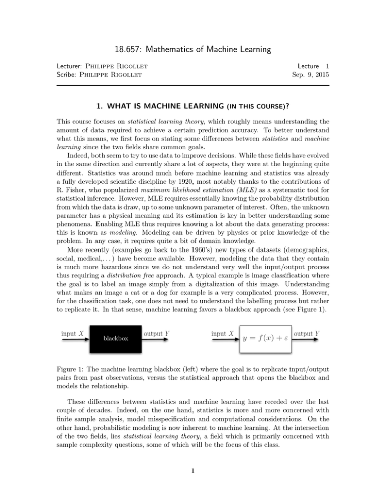
to replicate it. In that sense, machine learning favors a blackbox approach (see Figure 1).
input X
blackbox
output Y
input X
y = f (x) + ε
output Y
Figure 1: The machine learning blackbox (left) where the goal is to replicate input/output
pairs from past observations, versus the statistical approach that opens the blackbox and
models the relationship.
These differences between statistics and machine learning have receded over the last
couple of decades. Indeed, on the one hand, statistics is more and more concerned with
finite sample analysis, model misspecification and computational considerations. On the
other hand, probabilistic modeling is now inherent to machine learning. At the intersection
of the two fields, lies statistical learning theory, a field which is primarily concerned with
sample complexity questions, some of which will be the focus of this class.
1
2. STATISTICAL LEARNING THEORY
2.1 Binary classification
A large part of this class will be devoted to one of the simplest problem of statistical learning
theory: binary classification (aka pattern recognition [DGL96]). In this problem, we observe
(X1 , Y1 ), . . . , (Xn , Yn ) that are n independent random copies of (X, Y ) ∈ X × {0, 1}. Denote
by PX,Y the joint distribution of (X, Y ). The so-called feature X lives in some abstract
space X (think IRd ) and Y ∈ {0, 1} is called label. For example, X can be a collection of
gene expression levels measured on a patient and Y indicates if this person suffers from
obesity. The goal of binary classification is to build a rule to predict Y given X using
only the data at hand. Such a rule is a function h : X → {0, 1} called a classifier. Some
classifiers are better than others and we will favor ones that have low classification error
6 Y ). Let us make some important remarks.
R(h) = IP(h(X) =
Fist of all, since Y ∈ {0, 1} then Y has a Bernoulli distribution: so much for distribution
free assumptions! However, we will not make assumptions on the marginal distribution of
X or, what matters for prediction, the conditional distribution of Y given X. We write,
Y |X ∼ Ber(η(X)), where η(X) = IP(Y = 1|X) = IE[Y |X] is called the regression function
of Y onto X.
Next, note that we did not write Y = η(X). Actually we have Y = η(X) + ε, where
ε = Y −η(X) is a “noise” random variable that satisfies IE[ε|X] = 0. In particular, this noise
accounts for the fact that X may not contain enough information to predict Y perfectly.
This is clearly the case in our genomic example above: it not whether there is even any
information about obesity contained in a patient’s genotype. The noise vanishes if and only
if η(x) ∈ {0, 1} for all x ∈ X . Figure 2.1 illustrates the case where there is no noise and the
the more realistic case where there is noise. When η(x) is close to .5, there is essentially no
information about Y in X as the Y is determined essentially by a toss up. In this case, it
is clear that even with an infinite amount of data to learn from, we cannot predict Y well
since there is nothing to learn. We will see what the effect of the noise also appears in the
sample complexity.
η(x)
1
.5
x
Figure 2: The thick black curve corresponds to the noiseless case where Y = η(X) ∈ {0, 1}
and the thin red curve corresponds to the more realistic case where η ∈ [0, 1]. In the latter
case, even full knowledge of η does not guarantee a perfect prediction of Y .
In the presence of noise, since we cannot predict Y accurately, we cannot drive the
classification error R(h) to zero, regardless of what classifier h we use. What is the smallest
value that can be achieved? As a thought experiment, assume to begin with that we have all
2
the information that we may ever hope to get, namely we know the regression function η(·).
For a given X to classify, if η(X) = 1/2 we may just toss a coin to decide our prediction
and discard X since it contains no information about Y . However, if η(X) =
6 1/2, we have
an edge over random guessing: if η(X) > 1/2, it means that IP(Y = 1|X) > IP(Y = 0|X)
or, in words, that 1 is more likely to be the correct label. We will see that the classifier
h∗ (X) = 1I(η(X) > 1/2) (called Bayes classifier ) is actually the best possible classifier in
the sense that
R(h∗ ) = inf R(h) ,
h(·)
where the infimum is taken over all classifiers, i.e. functions from X to {0, 1}. Note that
unless η(x) ∈ {0, 1} for all x ∈ X (noiseless case), we have R(h∗ ) =
6 0. However, we can
always look at the excess risk E(h) of a classifier h defined by
E(h) = R(h) − R(h∗ ) ≥ 0 .
In particular, we can hope to drive the excess risk to zero with enough observations by
mimicking h∗ accurately.
2.2 Empirical risk
The Bayes classifier h∗ , while optimal, presents a major drawback: we cannot compute it
because we do not know the regression function η. Instead, we have access to the data
(X1 , Y1 ), . . . , (Xn , Yn ), which contains some (but not all) information about η and thus h∗ .
In order to mimic the properties of h∗ recall that it minimizes R(h) over all h. But the
function R(·) is unknown since it depends on the unknown distribution PX,Y of (X, Y ). We
ˆ n (·) defined for
estimate it by the empirical classification error, or simply empirical risk R
any classifier h by
n
1X
R̂n (h) =
1I(h(Xi ) 6= Yi ) .
n
i=1
ˆ n (h)] = R(h) so R
ˆ n (h) is
Since IE[1I(h(Xi ) 6= Yi )] = IP(h(Xi ) 6= Yi ) = R(h), we have IE[R
an unbiased estimator of R(h). Moreover, for any h, by the law of large numbers, we have
ˆ n (h) → R(h) as n → ∞, almost surely. This indicates that if n is large enough, R
ˆ n (h)
R
should be close to R(h).
As a result, in order to mimic the performance of h∗ , let us use the empirical risk
ˆ defined to minimize R
ˆ n (h) over all classifiers h. This is an easy enough
minimizer (ERM) h
ˆ such h(X
ˆ i ) = Yi for all i = 1, . . . , n and h(x) = 0 if x ∈
task: define h
/ {X1 , . . . , Xn }. We
ˆ
ˆ
have Rn (h) = 0, which is clearly minimal. The problem with this classifier is obvious: it
does not generalize outside the data. Rather, it predicts the label 0 for any x that is not in
ˆ = 0.
ˆ n (h)
the data. We could have predicted 1 or any combination of 0 and 1 and still get R
ˆ
In particular it is unlikely that IE[R(h)] will be small.
3
Important Remark: Recall that R(h) = IP(h(X) 6= Y ).
ˆ = h({(X
ˆ
ˆ
If h(·)
1 , Y1 ), . . . , (Xn , Yn )} ; ·) is constructed from the data, R(h) denotes
the conditional probability
ˆ = IP(h(X)
ˆ
R(h)
6= Y |(X1 , Y1 ), . . . , (Xn , Yn )) .
ˆ
ˆ is a random variable since it depends on the
rather than IP(h(X)
6= Y ). As a result R(h)
randomness of the data (X1 , Y1 ), . . . , (Xn , Yn ). One way to view this is to observe that
ˆ
we compute the deterministic function R(·) and then plug in the random classifier h.
This problem is inherent to any method if we are not willing to make any assumption
on the distribution of (X, Y ) (again, so much for distribution freeness!). This can actually
be formalized in theorems, known as no-free-lunch theorems.
ˆ built from (X1 , Y1 ), . . . , (Xn , Yn ) and
Theorem: For any integer n ≥ 1, any classifier h
any ε > 0, there exists a distribution PX,Y for (X, Y ) such that R(h∗ ) = 0 and
ˆ n ) ≥ 1/2 − ε .
IER(h
To be fair, note that here the distribution of the pair (X, Y ) is allowed to depend on
n which is cheating a bit but there are weaker versions of the no-free-lunch theorem that
essentially imply that it is impossible to learn without further assumptions. One such
theorem is the following.
ˆ built from (X1 , Y1 ), . . . , (Xn , Yn ) and any sequence
Theorem: For any classifier h
{an }n > 0 that converges to 0, there exists a distribution PX,Y for (X, Y ) such that
R(h∗ ) = 0 and
ˆ n ) ≥ an , for all n ≥ 1
IER(h
In the above theorem, the distribution of (X, Y ) is allowed to depend on the whole sequence
{an }n > 0 but not on a specific n. The above result implies that the convergence to zero of
the classification error may be arbitrarily slow.
2.3 Generative vs discriminative approaches
Both theorems above imply that we need to restrict the distribution PX,Y of (X, Y ). But
isn’t that exactly what statistical modeling is? The is answer is not so clear depending on
how we perform this restriction. There are essentially two schools: generative which is the
statistical modeling approach and discriminative which is the machine learning approach.
Generative: This approach consists in restricting the set of candidate distributions PX,Y .
This is what is done in discriminant analysis 1 where it is assumed that the condition dis1
Amusingly, the generative approach is called discriminant analysis but don’t let the terminology fool
you.
4
tributions of X given Y (there are only two of them: one for Y = 0 and one for Y = 1) are
Gaussians on X = IRd (see for example [HTF09] for an overview of this approach).
Discriminative: This is the machine learning approach. Rather than making assumptions
directly on the distribution, one makes assumptions on what classifiers are likely to perform
correctly. In turn, this allows to eliminate classifiers such as the one described above and
that does not generalize well.
While it is important to understand both, we will focus on the discriminative approach
in this class. Specifically we are going to assume that we are given a class H of classifiers
such that R(h) is small for some h ∈ H.
2.4 Estimation vs. approximation
Assume that we are given a class H in which we expect to find a classifier that performs well.
This class may be constructed from domain knowledge or simply computational convenience.
ˆ n built from the data,
We will see some examples in the class. For any candidate classifier h
we can decompose its excess risk as follows:
ˆ n ) = R(h
ˆ n ) − R(h∗ ) = R(h
ˆ n ) − inf R(h) + inf R(h) − R(h∗ ) .
E(h
h∈H
h∈H
|
{z
} |
{z
}
estimation error
approximation error
On the one hand, estimation error accounts for the fact that we only have a finite
amount of observations and thus a partial knowledge of the distribution PX,Y . Hopefully
we can drive this error to zero as n → ∞. But we already know from the no-free-lunch
theorem that this will not happen if H is the set of all classifiers. Therefore, we need to
take H small enough. On the other hand, if H is too small, it is unlikely that we will
find classifier with performance close to that of h∗ . A tradeoff between estimation and
approximation can be made by letting H = Hn grow (but not too fast) with n.
For now, assume that H is fixed. The goal of statistical learning theory is to understand
how the estimation error drops to zero as a function not only of n but also of H. For the
first argument, we will use concentration inequalities such as Hoeffding’s and Bernstein’s
inequalities that allow us to control how close the empirical risk is to the classification error
by bounding the random variable
n
1 X
1I(h(Xi ) =
6 Yi ) − IP(h(X) =
6 Y )
n
i=1
with high probability. More generally we will be interested in results that allow to quantify
how close the average of independent and identically distributed (i.i.d) random variables is
to their common expected value.
ˆ ≤R
ˆ n (h)
ˆ n (h) for all h ∈ H, the estimation error
Indeed, since by definition, we have R
¯
can be controlled as follows. Define h ∈ H to be any classifier that minimizes R(·) over H
(assuming that such a classifier exist).
ˆ n ) − inf R(h) = R(h
ˆ n ) − R(h)
¯
R(h
h∈H
ˆ )−R
¯ +R(h
ˆ n ) − R̂n (h
ˆ n ) + R̂n (h)
¯ − R(h)
¯
ˆ (h
ˆ (h)
=R
| n n {z n }
≤0
ˆ n ) − R(h
ˆ n ) + R
¯ − R(h)
¯ .
ˆ n (h
ˆ n (h)
≤ R
5
¯ is deterministic, we can use a concentration inequality to control R
¯ − R(h)
¯ .
ˆ n (h)
Since h
However,
n
X
ˆn) = 1
ˆ n (Xi ) 6= Yi )
ˆ n (h
R
1I(h
n
i=1
ˆ n depends in a complicated
is not the average of independent random variables since h
manner on all of the pairs (Xi , Yi ), i = 1, . . . , n. To overcome this limitation, we often use
ˆ n,
a blunt, but surprisingly accurate tool: we “sup out” h
ˆ n ) − R(h
ˆ n ) ≤ sup R
ˆ n ) − R(h
ˆ n ) .
R
ˆ n (h
ˆ n (h
h∈H
Controlling this supremum falls in the scope of suprema of empirical processes that we will
study in quite a bit of detail. Clearly the supremum is smaller as H is smaller but H should
be kept large enough to have good approximation properties. This is the tradeoff between
approximation and estimation. It is also know in statistics as the bias-variance tradeoff.
References
[DGL96] L. Devroye, L. Györfi, and G. Lugosi, A probabilistic theory of pattern recognition,
Applications of Mathematics (New York), vol. 31, Springer-Verlag, New York,
1996. MR MR1383093 (97d:68196)
[HTF09] Trevor Hastie, Robert Tibshirani, and Jerome Friedman, The elements of statistical learning, second ed., Springer Series in Statistics, Springer, New York, 2009,
Data mining, inference, and prediction. MR 2722294 (2012d:62081)
6
MIT OpenCourseWare
http://ocw.mit.edu
18.657 Mathematics of Machine Learning
Fall 2015
For information about citing these materials or our Terms of Use, visit: http://ocw.mit.edu/terms.