Lecture 27
Application of Martingale inequalities. Generalized Martingale inequalities.
18.465
�
�
�n
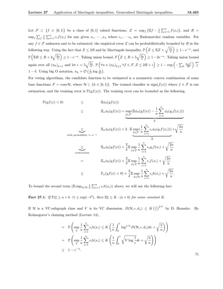
Let F ⊂ {f ∈ [0, 1]} be a class of [0, 1] valued functions, Z = supf Ef − n1 i=1 f (xi ) , and R =
�
�n
supf f n1 i=1 �i f (xi ) for any given xi , · · · , xn where �1 , · · · �n are Rademarcher random variables. For
any f ∈ F unknown and to be estimated, the empirical error Z can be probabilistically bounded by R in the
� �
�
following way. Using the fact that Z ≤ 2R and by Martingale inequality, P Z ≤ EZ + 2u
≥ 1 − e−u , and
n
� �
� �
�
�
P ER ≤ R + 2 2nu ≥ 1 − e−u . Taking union bound, P Z ≤ R + 5 2nu ≥ 1 − 2e−u . Taking union bound
�
�
�
� �
� set
n k �2
again over all (nk )k>1 and let � = 5 2u
,
P
∀n
∈
(n
)
∀f
∈
F,
Z
≤
2R
+
�
≥
1
−
exp
−
≥
k
k≥1
k 50
n
�1
�
1
1 − δ. Using big O notation, nk = O �2 log δ2 .
For voting algorithms, the candidate function to be estimated is a symmetric convex combination of some
base functions F = convH, where H ⊂ {h ∈ [0, 1]}. The trained classifier is sign(f (x)) where f ∈ F is our
estimation, and the training error is P(yf (x)). The training error can be bounded as the following,
P(yf (x) < 0)
≤
Eφδ (yf (x))
≤
En φδ (yf (x)) + sup (Eφδ (yf (x)) −
n
1�
φδ (yi f (xi )))
n i=1
��
�
f ∈F
�
≤
����
with probability 1−e−u
Z
n
1�
En φδ (yf (x)) + 2 · E sup(
�i φδ (yi f (xi ))) +
f ∈F n i=1
�
��
�
�
2u
n
R
2
1
En φδ (yf (x)) + E sup
δ f ∈F n
≤
����
contraction
n
�
�
�i yi f (xi ) +
i=1
n
2
1�
En φδ (yf (x)) + E sup
�i f (xi ) +
δ f ∈F n i=1
�
2u
n
�
n
2
1�
2u
Pn (yf (x) < 0) + E sup
�i h(xi ) +
.
n
δ h∈H n i=1
=
≤
To bound the second term (E suph∈H
2u
n
1
n
�n
i=1 �i h(xi ))
above, we will use the following fact.
Fact 27.1. If P(ξ ≥ a + b · t) ≤ exp(−t2 ), then Eξ ≤ K · (a + b) for some constant K.
If H is a VC-subgraph class and V is its VC dimension, D(H, �, dx ) ≤ K
� 1 �2·V
�
by D. Haussler. By
Kolmogorov’s chaining method (Lecture 14),
�
=
=
� ��
� � 1
n
1
u
1�
1/2
P sup
�i h(xi ) ≤ K
log D(H, �, dx )d� +
n 0
n
h n i=1
�
�
��
�
�
�
n
1 1
1
u
1�
V log d� +
P sup
�i h(xi ) ≤ K
n 0
�
n
h n i=1
≥ 1 − e−u .
71
Lecture 27
Application of Martingale inequalities. Generalized Martingale inequalities.
Thus E sup n1
�
�i h(xi ) ≤ K
��
V
n
+
� �
1
n
≤K
�
V
n,
18.465
and
�
1
P P(yf (x) < 0) ≤ Pn (yf (x) < 0) + K
δ
�
V
+
n
�
2u
n
�
≥ 1 − e−u .
Recall our set up for Martingale inequalities. Let Z = Z(x1 , · · · , xn ) where x1 , · · · , xn are independent
random variables. We need to bound Z − EZ. Since Z is not a sum of independent random variables, certain
classical concentration inequalities is not applicable. But we can try to bound Z − EZ with certain form of
Martingale inequalities.
Z − EZ
= Z − Ex1 (Z |x2 , · · · , xn ) + Ex1 (Z|x2 , · · · , xn ) − Ex1 ,x2 (Z|x3 , · · · , xn ) +
�
��
� �
��
�
d1 (x1 ,··· ,xn )
d2 (x2 ,··· ,xn )
· · · + Ex1 ,··· ,xn−1 (Z |xn ) − Ex1 ,··· ,xn (Z)
�
��
�
dn (xn )
with the assumptions that Exi di = 0, and �di �∞ ≤ ci .
�n
We will give a generalized martingale inequality below.
maxi �di �∞ ≤ C,
σi2
=
σi2 (xi+1 , · · ·
i=1
di = Z − EZ where di = di (xi , · · · , xn ),
, xn ) = var(di ), and Edi = 0. Take � > 0,
n
n
�
�
P(
di − �
σi2 ≥ t)
i=1
i=1
n
�
≤ e−λt E exp(
λ(di − �σi2 ))
i=1
=
e−λt E exp(
n−1
�
λ(di − �σi2 ) · E exp(λdn ) · exp(λ�σn2 )
i=1
The term exp(λdn ) can be bounded in the following way.
=
����
E exp(λdn )
�
�
λ2 2 λ3 3
E 1 + λdn + dn + dn + · · ·
2!
3!
Taylor expansion
≤
≤
Choose λ such that
λ2
2·(1−λC)
�
�
λ2 2
λC
λ2 C 2
1 + σn · 1 +
+
+ ···
2
3
3·4
� 2 2
�
λ · σn
1
exp
·
.
2
(1 − λC)
≤ λ�, we get λ ≤
2�
1+2�C ,
and Edn exp(λdn ) · exp(λ�σn2 ) ≤ 1. Iterate over
i = n, · · · , 1, we get
P
� n
�
i=1
di − �
n
�
�
σi2
≥t
≤ exp (−λ · t)
i=1
72
Lecture 27
Application of Martingale inequalities. Generalized Martingale inequalities.
18.465
. Take t = u/λ, we get
P
� n
�
di ≥ �
i=1
To minimize the sum �
�n
i=1
σi2 +
u
2� (1
n
�
i=1
σi2
�
u
+ (1 + 2�C)
2�
≤ exp (−u)
+ 2�C), we set its derivative to 0, and get � =
�
2
u
P
σi2
. Thus
⎛
⎞
� �
�
P⎝
di ≥ 3 u
σi2 /2 + Cu⎠ ≤ e−u
i
. This inequality takes the form of the Bernstein’s inequality.
73