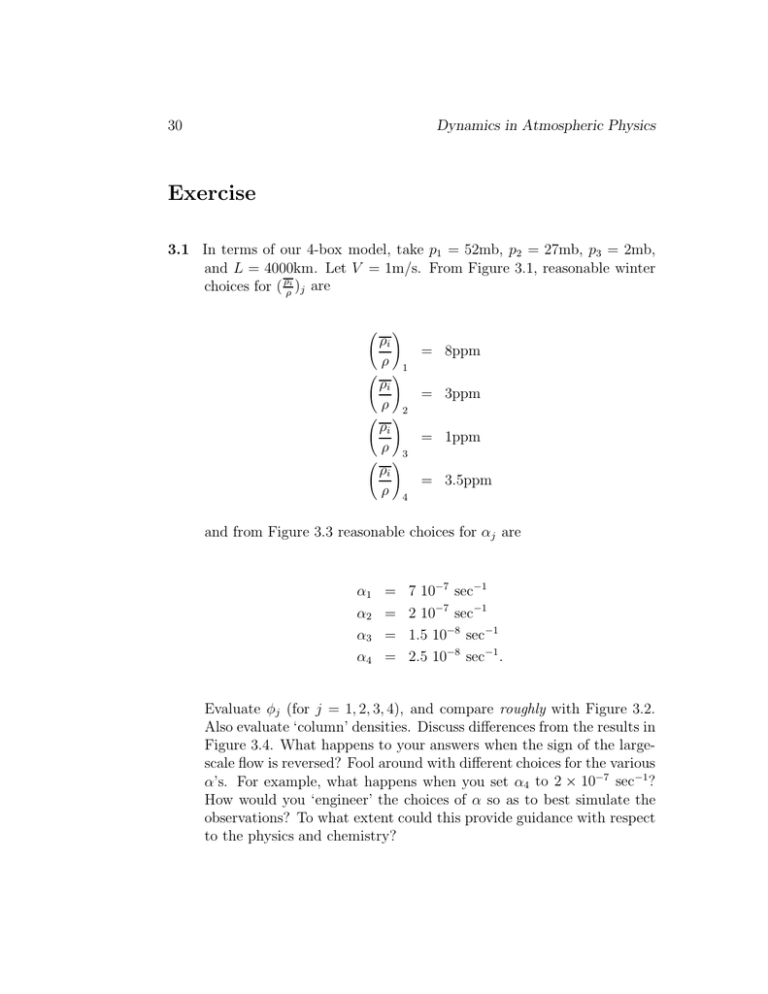
30
Dynamics in Atmospheric Physics
Exercise
3.1 In terms of our 4-box model, take p1 = 52mb, p2 = 27mb, p3 = 2mb,
and L = 4000km. Let V = 1m/s. From Figure 3.1, reasonable winter
choices for ( ρρi )j are
�
ρi
ρ
�
�
ρi
ρ
�
�
ρi
ρ
�
�
ρi
ρ
�
= 8ppm
1
= 3ppm
2
= 1ppm
3
= 3.5ppm
4
and from Figure 3.3 reasonable choices for αj are
α1
α2
α3
α4
=
=
=
=
7 10−7 sec−1
2 10−7 sec−1
1.5 10−8 sec−1
2.5 10−8 sec−1 .
Evaluate φj (for j = 1, 2, 3, 4), and compare roughly with Figure 3.2.
Also evaluate ‘column’ densities. Discuss differences from the results in
Figure 3.4. What happens to your answers when the sign of the largescale flow is reversed? Fool around with different choices for the various
α’s. For example, what happens when you set α4 to 2 × 10−7 sec−1?
How would you ‘engineer’ the choices of α so as to best simulate the
observations? To what extent could this provide guidance with respect
to the physics and chemistry?
Effect of transport on composition
31
Figure 3.7: 6-box model.
Note that the bottom of the 4-box model is at 52mb which does not
include the bulk of the lower region in Figure 3.2 where the reversal in
the meridional gradient of ozone occurs. Thus, the column densities are
not expected to replicate those in Figure 3.4. If, instead of our 4-box
model, we had a 6-box model of the sort shown in Figure 3.7we could
choose the bottom to be at 100mb. Try to rig the properties of the 6
boxes (while not choosing values which are too unrealistic) in order to
match Figure 3.4. What is needed? Again, try to ‘engineer’ choices
of parameters to achieve a best simulation. Discuss the limitations of
these models.