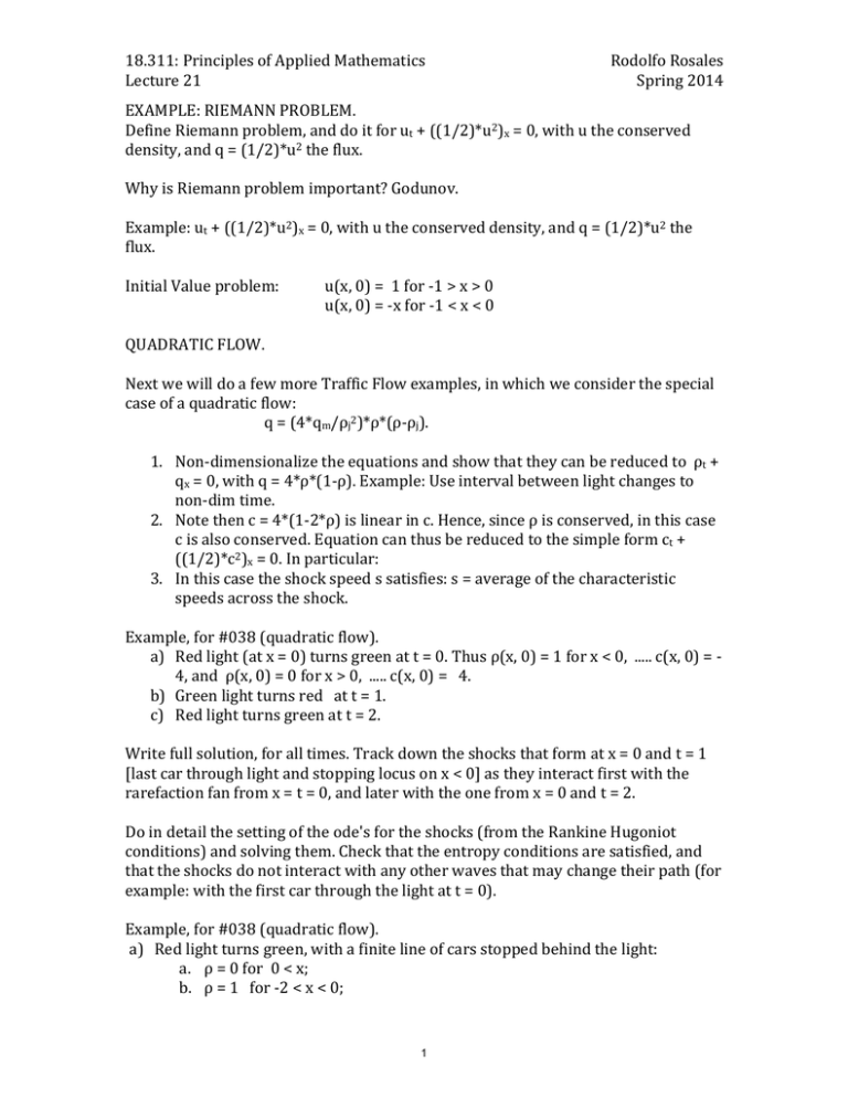
18.311: Principles of Applied Mathematics Lecture 21 Rodolfo Rosales Spring 2014 EXAMPLE: RIEMANN PROBLEM. Define Riemann problem, and do it for ut + ((1/2)*u2)x = 0, with u the conserved density, and q = (1/2)*u2 the flux. Why is Riemann problem important? Godunov. Example: ut + ((1/2)*u2)x = 0, with u the conserved density, and q = (1/2)*u2 the flux. Initial Value problem: u(x, 0) = 1 for -­‐1 > x > 0 u(x, 0) = -­‐x for -­‐1 < x < 0 QUADRATIC FLOW. Next we will do a few more Traffic Flow examples, in which we consider the special case of a quadratic flow: q = (4*qm/ρj2)*ρ*(ρ-­‐ρj). 1. Non-­‐dimensionalize the equations and show that they can be reduced to ρt + qx = 0, with q = 4*ρ*(1-­‐ρ). Example: Use interval between light changes to non-­‐dim time. 2. Note then c = 4*(1-­‐2*ρ) is linear in c. Hence, since ρ is conserved, in this case c is also conserved. Equation can thus be reduced to the simple form ct + ((1/2)*c2)x = 0. In particular: 3. In this case the shock speed s satisfies: s = average of the characteristic speeds across the shock. Example, for #038 (quadratic flow). a) Red light (at x = 0) turns green at t = 0. Thus ρ(x, 0) = 1 for x < 0, ..... c(x, 0) = -­‐ 4, and ρ(x, 0) = 0 for x > 0, ..... c(x, 0) = 4. b) Green light turns red at t = 1. c) Red light turns green at t = 2. Write full solution, for all times. Track down the shocks that form at x = 0 and t = 1 [last car through light and stopping locus on x < 0] as they interact first with the rarefaction fan from x = t = 0, and later with the one from x = 0 and t = 2. Do in detail the setting of the ode's for the shocks (from the Rankine Hugoniot conditions) and solving them. Check that the entropy conditions are satisfied, and that the shocks do not interact with any other waves that may change their path (for example: with the first car through the light at t = 0). Example, for #038 (quadratic flow). a) Red light turns green, with a finite line of cars stopped behind the light: a. ρ = 0 for 0 < x; b. ρ = 1 for -­‐2 < x < 0; 1
18.311: Principles of Applied Mathematics Lecture 21 Rodolfo Rosales Spring 2014 c. ρ = 1/2 for x < -­‐2; d. Solve using characteristics. Then plug in expansion fans and shocks. b) Let the light turn back to red at t = T > 1. Continue the solution. a. Identify shocks that correspond to car paths (last car through light) and check shock speed = u for them. c) Let the light turn back to green at t = 2*T. Continue solution. EXAMPLE, a signaling problem. Solve ut + u*ux = 0 on x > 0 with: • u(0, t) = 1 for t < 0; • u(0, t) = 1/2 for t > 0; Yet another recap on the laws governing shocks/hydraulic jumps. IMPORTANT: Shocks are not always the answer to wave breakdown and multiple values. Shocks introduce new physics. Without shocks, system is reversible. With shocks, system is not reversible. Physics needed to get shocks: flow against gradient and locality. • Rankine Hugoniot jump conditions for shocks and integral form of the conservation laws. s = [q]/[ρ]. Recall simple derivation using conservation in shock frame, where flux is (u-­‐s)*ρ. Hence ((u-­‐s)*ρ)-­‐ = ((u-­‐s)*ρ)+. • Shocks are curves in space time along which characteristics end, so crossing does no occur. They are NOT NEEDED OTHERWISE! Shocks MUST satisfy the ENTROPY condition: c-­‐ > s > c+. At a discontinuity where c+ < c-­‐, insert an EXPANSION FAN, not a shock. • Arrow of time and causality: characteristics die at shock, hence INFORMATION IS LOST. Irreversible evolution, FORWARD IN TIME ONLY. Entropy involves death (of characteristics, at shocks). • The entropy condition allows causality, with the shock (and the solution on each side) determined by the data (see next). • Assume piecewise smooth solution with shocks. At a shock, the problem splits into three subproblems: -­‐ Solution ahead of the shock. Smooth and satisfying characteristic form. Determined at each point by a single characteristic connecting to data. -­‐ Solution behind the shock: same deal as solution ahead of shock. -­‐ Shock position determined by solving o.d.e. given by jump cond. • The shock conditions in the Q-­‐ρ Flow-­‐Density plane. 2
18.311: Principles of Applied Mathematics Lecture 21 -­‐
-­‐
-­‐
Rodolfo Rosales Spring 2014 Need consistency between entropy condition and jump condition. Jump condition must yield shock velocity satisfying c-­‐ > s > c+. Works for for Q concave or convex. More complicated otherwise. FOR NOW WE ONLY CONSIDER SITUATIONS WHERE THE FLUX IS CONVEX OR CONCAVE. Traffic flow: backward facing shocks, moving slower than cars. Car enter shock region from behind. (Q concave). River flow: forward facing shocks, moving faster than water flow. Water enters hydraulic jumps from ahead. 3
MIT OpenCourseWare
http://ocw.mit.edu
18.311 Principles of Applied Mathematics
Spring 2014
For information about citing these materials or our Terms of Use, visit: http://ocw.mit.edu/terms.