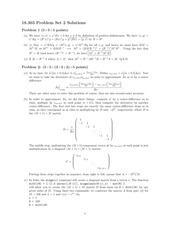
18.303 Problem Set 2 Solutions
Problem 1 (5+5+5 points)
(a) We have (x, x) = x∗ Bx > 0 for x = 0 by definition of positive-definiteness. We have (x, y) =
x∗ By = (B ∗ x)∗ y = (Bx)∗ y = y ∗ (Bx) = (y, x) by B = B ∗ .
(b) (x, M y) = x∗ BM y = (M † x, y) = x∗ M †∗ By for all x, y, and hence we must have BM =
M †∗ B, or M †∗ = BM B −1 =⇒ M † = (BM B −1 )∗ = (B −1 )∗ M ∗ B ∗ . Using the fact that
B ∗ = B (and hence (B −1 )∗ = B −1 ), we have M † = B −1 M ∗ B .
(c) If M = B −1 A where A = A∗ , then M † = B −1 AB −1 B = B −1 A = M . Q.E.D.
Problem 2: (5+5+(3+3+3)+5 points)
−um
(a) As in class, let u' ([m + 0.5]Δx) ≈ u'm+0.5 = um+1
. Define cm+0.5 = c([m + 0.5]Δx). Now
Δx
'
ˆ at m by a center
we want to take the derivative of cm+0.5 um+0.5 in order to approximate Au
difference:
−um
m−1
cm+0.5 um+1
− cm−0.5 um −u
Δx
Δx
Âu
≈
.
Δx
mΔx
There are other ways to solve this problem of course, that are also second-order accurate.
ˆ we did three things: compute u' by a center-difference as in
(b) In order to approximate Au,
class, multiply by cm+0.5 at each point m + 0.5, then compute the derivative by another
center-difference. The first and last steps are exactly the same center-difference steps as in
class, so they correspond as in class to multiplying by D and −DT , respectively, where D is
the (M + 1) × M matrix
⎛
⎞
1
⎜ −1 1
⎟
⎜
⎟
⎜
⎟
−1 1
1 ⎜
⎟
D=
⎜
⎟.
.
.
.
.
⎟
⎜
Δx
.
.
⎟
⎜
⎝
−1 1 ⎠
−1
The middle step, multiplying the (M + 1)-component vector u' by cm+0.5 at each point is just
multiplication by a diagonal (M + 1) × (M + 1) matrix
⎛
⎞
c0.5
⎜
⎟
c1.5
⎜
⎟
C=⎜
⎟.
..
⎝
⎠
.
cM +0.5
Putting these steps together in sequence, from right to left, means that A = −DT CD
(c) In Julia, the diagm(c) command will create a diagonal matrix from a vector c. The function
diff1(M) = [ [1.0 zeros(1,M-1)]; diagm(ones(M-1),1) - eye(M) ]
will allow you to create the (M + 1) × M matrix D from class via D = diff1(M) for any
given value of M . Using these two commands, we construct the matrix A from part (d) for
M = 100 and L = 1 and c(x) = e3x via
L = 1 M = 100
D = diff1(M)
1
0.20
fourth
third
0.15
second
first
eigenfunctions
0.10
0.05
0.00
0.05
0.10
0.15
0.20
0.0
0.2
0.4
0.6
0.8
1.0
x
Figure 1: Smallest-|λ| eigenfunctions of  =
d
dx
d
c(x) dx
for c(x) = e3x .
dx = L / (M+1)
x = dx*0.5:dx:L # sequence of x values from 0.5*dx to <= L in steps of dx
c(x) = exp(3x)
C = diagm(c(x))
A = -D’ * C * D / dx^2
You can now get the eigenvalues and eigenvectors by λ, U = eig(A), where λ is an array of
eigenvalues and U is a matrix whose columns are the corresponding eigenvectors (notice that
all the λ are < 0 since A is negative-definite).
(i) The plot is shown in Figure 1. The eigenfunctions look vaguely “sine-like”—they have
the same number of oscillations as sin(nπx/L) for n = 1, 2, 3, 4—but are “squeezed” to
the left-hand side.
(ii) We find that the dot product is ≈ 4.3 × 10−16 , which is zero up to roundoff errors (your
exact value may differ, but should be of the same order of magnitude).
(iii) In the posted IJulia notebook for the solutions, we show a plot of |λ2M −λM | as a function
of M on a log–log scale, and verify that it indeed decreases ∼ 1/M 2 . You can also just
look at the numbers instead of plotting, and we find that this difference decreases by a
factor of ≈ 3.95 from M = 100 to M = 200 and by a factor of ≈ 3.98 from M = 200 to
M = 400, almost exactly the expected factor of 4. (For fun, in the solutions I went to
M = 1600, but you only needed to go to M = 800.)
(d) In general, the eigenfunctions have the same number of nodes (sign oscillations) as sin(nπx/L),
but the oscillations pushed towards the region of high c(x). This is even more dramatic if we
increase the c(x) contrast. In Figure xxx, we show two examples. First, c(x) = e20x , in which
all of the functions are squished to the left where c is small. Second c(x) = 1 for x < 0.3
and 100 otherwise—in this case, the oscillations are at the left 1/3 where c is small, but the
function is not zero in the right 2/3. Instead, the function is nearly constant where c is large.
The reason for this has to do with the continuity of u: it is easy to see from the operator that
cu' must be continuous for (cu' )' to exist, and hence the slope u' must decrease by a factor of
2
ˆ = (cu' )' for two different choices of c(x).
Figure 2: First four eigenfunctions of Au
100 for x > 0.3, leading to a u that is nearly constant. (We will explore some of these issues
further later in the semester.)
Problem 3: (5+5+5+5+5+5 points)
dQn
1
n
(a) The heat capacity equation tells us that dT
dt = cρaΔx dt , where dQn /dt is the rate of change
of the heat in the n-th piece. The thermal conductivity equation tells us that dQn /dt, in
turn, is equal to the sum of the rates q at which heat flows from n + 1 and n − 1 into n:
1 dQn
1
κa
dTn
=
=
[(Tn+1 − Tn ) + (Tn−1 − Tn )] = α(Tn+1 −Tn )+α(Tn−1 −Tn )
dt
cρaΔx dt
cρaΔx Δx
where α =
κ
. The only difference for T1 and TN is that they have no heat flow
cρ(Δx)2
n − 1 and n + 1, respectively, since the ends are insulated:
α(TN −1 − TN ).
dT1
dt
= α(T2 − T1 ) and
dTN
dt
=
(b) We can obtain A in two ways. First, we can simply look directly at our equations above,
n
which give dT
dt = α(Tn+1 − 2Tn + Tn−1 ) for every n except T1 and TN , and read off the
3
corresponding rows of the matrix
⎛
−1
⎜ 1
⎜
⎜
A = α⎜
⎜
⎝
1
−2
..
.
⎞
1
..
.
1
..
.
−2
1
⎟
⎟
⎟
⎟.
⎟
1 ⎠
−1
Alternatively, we can write each of the above steps—differentiating T to get the rate of heat
flow q to the left at each of the N − 1 interfaces between the pieces, then taking the difference
of the q’s to get dT /dt, in matrix form, to write:
⎛
⎞
⎛
⎞
1
−1 1
⎜ −1 1
⎟
⎜
⎟
⎜
⎟
−1 1
⎟
⎟
−1 1
1 1 ⎜
1 ⎜
κ
⎜
⎟
⎜
⎟
..
..
A=
κa
⎜
⎟
⎜
⎟ = − DDT ,
.
.
.
.
..
..
⎟ Δx ⎜
⎟
cρa Δx ⎜
cρ
⎜
⎟
⎝
⎠
−1 1
⎝
−1 1 ⎠
−1 1
−1
__
_
__
_
−D T : (N −1)×N
D: N ×(N −1)
in terms of the D matrix from class (except with N reduced by 1), which gives the same A
as above. As we will see in the parts below, this is indeed a second-derivative approximation,
but with different boundary conditions—Neumann conditions—than the Dirichlet conditions
in class.
By the way, it is interesting to consider −DDT , compared to the −DT D we had in class.
Clearly, −DDT is real-symmetric and negative semidefinite. It is not, however, negative def­
inite, since DT does not (and cannot) have full column rank (its rank must be ≤ the number
of rows N − 1, and in fact in class we showed that it has rank N − 1).
dTn
dt
κ ∂2T
cρ ∂x2
(c) Ignoring the ends for the moment, for all the interior points we have
which is exactly our familiar center-difference approximation for
=
at the point n (x =
[n − 0.5]Δx). Hence, everywhere in the interior our equations converge to
thus  =
κ Tn+1 −2Tn +Tn−1
,
cρ
Δx2
∂T
∂T
=
κ ∂2T
cρ ∂x2
, and
2
κ ∂
.
cρ ∂x2
∂T
= 0 at x = 0, L. The easiest way to see this is to
∂x
observe that our heat flow q is really a first derivative, and zero heat flow at the ends
−Tn
means zero derivatives.
That is, qn+0.5 = κa Tn+1
is really an approximate derivative:
Δx
∂T ∂T qn+0.5 ≈ κa ∂x n+0.5 = κa ∂x nΔx , while the flows q0.5 and qN +0.5 to/from n = 0 and
n = N + 1 is zero, and hence q0.5 = qN +0.5 = 0 ≈ κa ∂T
∂x 0,L .
(d) The boundary conditions are
ˆ = ∂ 2 T2 = T '' (setting κ = 1 for convenience) with these
Working backwards, consider AT
∂x
cρ
boundary conditions and center-difference approximations.
We are given Tn = T ([n −
−Tn
'
0.5]Δx, t) for n = 1, . . . , N . First, we compute ∂T
≈
Tn+0.5
= Tn+1
for n =
∂x nΔx
Δx
T
1, . . . , N − 1 (−D T using the D above). Unlike the Dirichlet case in class, we don’t com­
'
pute T0.5
and TN' +0.5 , since these correspond to ∂T /∂x at x = 0, L, which are zero by the
boundary conditions. Then, we compute our approximate 2nd derivatives Tn'' =
4
−Tn−0.5
Tn+0.5
Δx
'
for n = 1, . . . , N , where we let T0.5
= TN'0 +0.5 = 0 (DT' using the D from above). This
0
0−TN −0.5
−0
T1.5
+TN −1
''
2 −T1
= TΔx
= −TNΔx
at the endpoints, and
2 , TN =
2
Δx
Δx
(Tn+1 −Tn )−(Tn −Tn−1 )
Tn+1 −2Tn +Tn−1
=
for 1 < n < N , which are precisely the rows of
Δx2
Δx2
gives T1'' =
Tn'' =
our A
matrix above.
(e) If κ(x), then we get a different κ and α factor for each Tn+1 − Tn difference:
dTn
= αn+1/2 (Tn+1 − Tn ) + αn−1/2 (Tn−1 − Tn ),
dt
where αn+1/2 =
κn+1/2
cρ(Δx)2
and κn+1/2 = κ([n + 1/2]Δx). In the N → ∞ limit, this gives
1 ∂ ∂
κ
: we differentiated, multiplied by κ, differentiated again, and then divided
cρ ∂x ∂x
by cρ. (You weren’t asked to handle the case where cρ is not a constant, so it’s okay if you
commuted cρ with the derivatives.)
 =
(f) If we discretize to Tm,n = T (mΔx, nΔy), the steps are basically the same except that we have
to consider the heat flow in both the x and y directions, and hence we have to take differences
in both x and y. In particular, suppose the thickness of the block is h. In this case, heat
will flow from Tm,n to Tm+1,n at a rate κhΔy
Δx (Tm,n − Tm+1,n ) where hΔy is the area of the
interface between the two blocks. Then, to convert into a rate of temperature change, we will
divide by cρhΔxΔy, where hΔxΔy is the volume of the block. Putting this all together, we
obtain:
κ Tm+1,n − 2Tm,n + Tm−1,n
Tm,n+1 − 2Tm,n + Tm,n+1
dTm,n
=
+
,
Δy 2
dt
cρ
Δx2
where the thing in [· · · ] is precisely the five-point stencil approximation for ∇2 from class.
Hence, we obtain
1
 = ∇ · κ∇,
cρ
where for fun I have put the κ in the middle, which is the right place if κ is not a constant
(you were not required to do this).
5
MIT OpenCourseWare
http://ocw.mit.edu
18.303 Linear Partial Differential Equations: Analysis and Numerics
Fall 2014
For information about citing these materials or our Terms of Use, visit: http://ocw.mit.edu/terms.