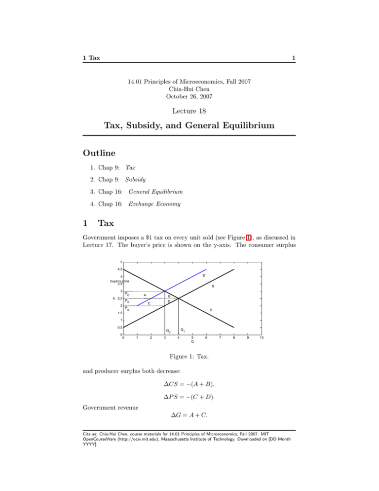
1 Tax
1
14.01 Principles of Microeconomics, Fall 2007
Chia-Hui Chen
October 26, 2007
Lecture 18
Tax, Subsidy, and General Equilibrium
Outline
1. Chap 9: Tax
2. Chap 9: Subsidy
3. Chap 16: General Equilibrium
4. Chap 16: Exchange Economy
1
Tax
Government imposes a $1 tax on every unit sold (see Figure 1), as discussed in
Lecture 17. The buyer’s price is shown on the y-axis. The consumer surplus
5
4.5
S’
4
buyer’s price
3.5
3
S
P
A
P
D
2.5
2
P0
B
D
C
P
D
S
1.5
1
0.5
0
Q
Q
1
0
0
1
2
3
4
5
Q
6
7
8
9
10
Figure 1: Tax.
and producer surplus both decrease:
ΔCS = −(A + B),
ΔP S = −(C + D).
Government revenue
ΔG = A + C.
Cite as: Chia-Hui Chen, course materials for 14.01 Principles of Microeconomics, Fall 2007. MIT
OpenCourseWare (http://ocw.mit.edu), Massachusetts Institute of Technology. Downloaded on [DD Month
YYYY].
2 Subsidy
2
So the deadweight loss is
DW L = B + D.
The burden of a tax is shared by consumers and producers; the relative amount
borne by consumers and producers depends on relative elasticities of demand
and supply.
• If the demand is inelastic (see Figure 2),
10
9
8
7
PD
S
P
6
5
P0
P
S
A
B
C
D
4
3
D
2
1
0
0
1
2
3
4
5
Q
6
7
8
9
10
Figure 2: Tax Burden on Buyers, Relative Inelastic Demand Curve.
ΔCS = −(A + B),
ΔP S = −(C + D),
buyers bear most of the burden of the tax.
• If the supply is inelastic (see Figure 3),
ΔCS = −(A + B),
ΔP S = −(C + D),
producers bear most of the burden of the tax.
Pass-through fraction is the percentage of a tax borne by consumers. It tells the
fraction of tax ”passed through” to consumers through higher price. If ED = 0,
say the demand is perfectly inelastic (see Figure 4), buyers bear all of the tax
burden:
ES
= 1.
ES − ED
Cite as: Chia-Hui Chen, course materials for 14.01 Principles of Microeconomics, Fall 2007. MIT
OpenCourseWare (http://ocw.mit.edu), Massachusetts Institute of Technology. Downloaded on [DD Month
YYYY].
2 Subsidy
3
10
9
8
S
7
P
6
P
D
P0
5
A
B
D
C
4
PS
3
D
2
1
0
0
2
4
6
8
10
Q
Figure 3: Tax Burden on Producers, Relative Inelastic Supply Curve.
Figure 4: Tax Burden on Buyers, Perfectly Inelastic Demand Curve.
Cite as: Chia-Hui Chen, course materials for 14.01 Principles of Microeconomics, Fall 2007. MIT
OpenCourseWare (http://ocw.mit.edu), Massachusetts Institute of Technology. Downloaded on [DD Month
YYYY].
2 Subsidy
4
5
4.5
4
S
3.5
P
3
2.5
2
PS
P
C
D
P
A
B
0
E
B
1.5
D
1
0.5
Q
0
Q
1
0
0
1
2
3
4
5
Q
6
7
8
9
10
Figure 5: Subsidy.
2
Subsidy
Government subsidizes $1 for each unit sold (see Figure 5). In this case, sellers’
price is higher than buyers’ price:
PB = PS + 1.
The consumer surplus increases by
ΔCS = A + B;
and the producer surplus increases by
ΔP S = C + D.
Government expenditure equals the whole area between PB and PS under the
quantity Q1
ΔG = −(A + B + C + D + E).
The deadweight loss is
DW L = E.
Likewise we can discuss the benefit of subsidy:
D
• if E
ES is small, namely, the demand is more inelastic, the benefit of subsidy
goes mostly to buyers;
D
• if E
ES is large, namely, the supply is more inelastic, the benefit of subsidy
goes mostly to sellers.
Cite as: Chia-Hui Chen, course materials for 14.01 Principles of Microeconomics, Fall 2007. MIT
OpenCourseWare (http://ocw.mit.edu), Massachusetts Institute of Technology. Downloaded on [DD Month
YYYY].
3 General Equilibrium
3
5
General Equilibrium
Partial equilibrium. Ignores effects form other markets.
General equilibrium. Simultaneous determination of the prices and quanti­
ties in all relevant markets, taking into account feedback effects.
Feedback effect. The price or quantity adjustment in one market caused by
price and quantity adjustments in related markets.
Example (DVD and Movie Tickets Markets). The price of a DVD is $3, and the
price of a movie ticket is $6 at equilibrium. Now tax $1 on the movie ticket (see
Figure 6). The specific process of price change is listed as follows:
MOVIE TICKET :
′
SM → SM
,
Price change:6 → 6.35;
DVD :
The price change of movie tickets shifts the demand curve of DVD.
DV → DV′ ,
Price change:3 → 3.5;
MOVIE TICKET :
The price change of DVD shifts the demand curve of movie tickets.
′
DM → DM
,
Price change:6.35 → 6.75;
and so on. The final equilibrium prices are
P (M OV IET ICKET ) = 6.85;
P (DV D) = 3.58.
If we ignore the feedback effects, we might underestimate the price change
bought by the tax.
Cite as: Chia-Hui Chen, course materials for 14.01 Principles of Microeconomics, Fall 2007. MIT
OpenCourseWare (http://ocw.mit.edu), Massachusetts Institute of Technology. Downloaded on [DD Month
YYYY].
3 General Equilibrium
6
10
9
SM*
8
SM
7
P
6
5
4
DM
3
2
1
0
0
2
4
6
8
10
Q
(a) Price Change of Movie Ticket.
10
9
8
7
SV
P
6
5
4
3
DV*
2
1
0
QV*
Q
V
0
1
2
3
4
5
Q
D
V
6
7
8
9
10
(b) Price Change of DVD.
Figure 6: General Equilibrium of DVD and Movie Ticket Markets.
Cite as: Chia-Hui Chen, course materials for 14.01 Principles of Microeconomics, Fall 2007. MIT
OpenCourseWare (http://ocw.mit.edu), Massachusetts Institute of Technology. Downloaded on [DD Month
YYYY].
4 Exchange Economy
4
7
Exchange Economy
Assume that:
• there are two consumers A and B;
• there are two goods, food and clothing;
• the quantities of food and clothing are 10 and 6, and A has 7 food and 1
clothing, while B has 3 food and 5 clothing;
• they know each others’ preferences;
• transaction cost is zero.
The edgeworth box is shown in Figure 7.
6
O
B
5
Clothing
4
3
2
1
A(7F,1C)=B(3F,5C)
OA
0
0
1
2
3
4
5
Food
6
7
8
9
10
Figure 7: Edgeworth Box.
Cite as: Chia-Hui Chen, course materials for 14.01 Principles of Microeconomics, Fall 2007. MIT
OpenCourseWare (http://ocw.mit.edu), Massachusetts Institute of Technology. Downloaded on [DD Month
YYYY].