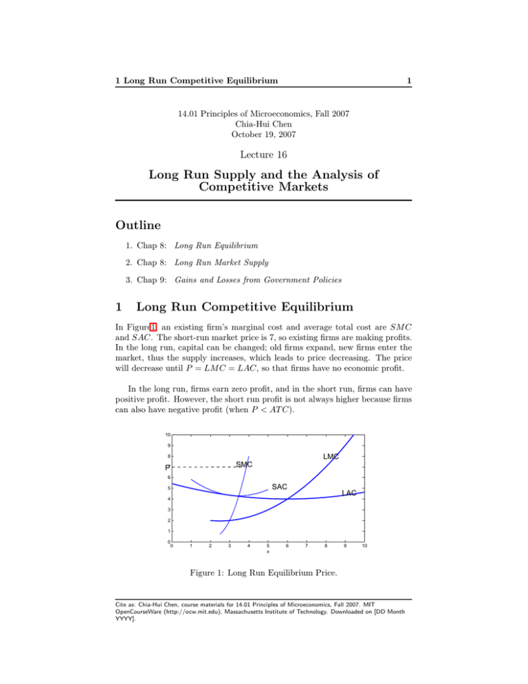
1 Long Run Competitive Equilibrium
1
14.01 Principles of Microeconomics, Fall 2007
Chia-Hui Chen
October 19, 2007
Lecture 16
Long Run Supply and the Analysis of
Competitive Markets
Outline
1. Chap 8: Long Run Equilibrium
2. Chap 8: Long Run Market Supply
3. Chap 9: Gains and Losses from Government Policies
1
Long Run Competitive Equilibrium
In Figure1, an existing firm’s marginal cost and average total cost are SM C
and SAC. The short-run market price is 7, so existing firms are making profits.
In the long run, capital can be changed; old firms expand, new firms enter the
market, thus the supply increases, which leads to price decreasing. The price
will decrease until P = LM C = LAC, so that firms have no economic profit.
In the long run, firms earn zero profit, and in the short run, firms can have
positive profit. However, the short run profit is not always higher because firms
can also have negative profit (when P < AT C).
10
9
LMC
8
SMC
P7
6
SAC
5
LAC
4
3
2
1
0
0
1
2
3
4
5
x
6
7
8
9
10
Figure 1: Long Run Equilibrium Price.
Cite as: Chia-Hui Chen, course materials for 14.01 Principles of Microeconomics, Fall 2007. MIT
OpenCourseWare (http://ocw.mit.edu), Massachusetts Institute of Technology. Downloaded on [DD Month
YYYY].
2 Long Run Market Supply
2
At long run competitive equilibrium:
• All firms are maximizing profit, or M R = M C.
• No firm has incentive to enter or exit earning zero economic profit (this is
the difference between short run and long run).
•
QD = QS .
In Figure 2, suppose the original price is 4. Existing firms make profit, so
new firms enter the market and the market supply curve shifts from S1 to S2 .
Now the market price is 3, existing firms make no profit, and new firms stop
entering. Thus, the equilibrium is reached.
In Figure 3, the original price 2 is lower than AC. Firms have a loss and
start leaving the market, and the market supply shifts from S1 to S2 .
5
5
4.5
4.5
S2
4
4
LAC
3.5
S1
3.5
3
3
2.5
2.5
2
2
LMC
1.5
1.5
1
1
0.5
0.5
0
0
0
0.5
1
1.5
2
2.5
3
3.5
4
4.5
5
D
0
0.5
1
1.5
2
2.5
3
3.5
4
4.5
5
4.5
5
Q
Q
(a) Long Run Cost.
(b) Shift of Equilibrium.
Figure 2: Long Run Equilibrium, High Price.
5
5
4.5
4.5
4
S1
3.5
3
3
2.5
2.5
2
2
LMC
1.5
1.5
1
1
0.5
0.5
0
S2
4
LAC
3.5
0
0.5
1
1.5
2
2.5
3
3.5
4
4.5
5
0
D
0
0.5
Q
(a) Long Run Cost.
1
1.5
2
2.5
3
3.5
4
Q
(b) Shift of Equilibrium.
Figure 3: Long Run Equilibrium, Low Price.
2
Long Run Market Supply
Assume that:
• All firms have the same technology;
• Initially firms produce at minimum long run average cost.
Cite as: Chia-Hui Chen, course materials for 14.01 Principles of Microeconomics, Fall 2007. MIT
OpenCourseWare (http://ocw.mit.edu), Massachusetts Institute of Technology. Downloaded on [DD Month
YYYY].
2 Long Run Market Supply
3
Constant-Cost Industry
In constant-cost industry, price of inputs does not change. If the price is higher
than minimum LAC. new firms will keep entering, so the supply is perfectly
elastic at P = minimumLAC. Long run supply is a horizontal line at the price
equal to the minimum LAC (see Figure 4(b)).
5
4
4.5
3.8
4
3.6
LAC
3.5
2
3
2.8
LMC
1.5
2.6
1
2.4
0.5
0
SL
P*
3.2
2.5
P
P
3.4
P*
3
2.2
Q*
0
0.5
1
1.5
2
2.5
Q
3
3.5
4
4.5
2
5
0
0.5
1
1.5
2
2.5
Q
3
3.5
4
4.5
5
(a) Long Run Cost in Constant-Cost In- (b) Supply Curve in Constant-Cost In­
dustry.
dustry.
Figure 4: Long Run Market Equilibrium in Constant-Cost Industry.
Increasing-Cost Industry
Price of some or all inputs rises as production is expanded and demand of inputs
increases. When the price increase from P ∗ to P ′ , firms are making profit. Old
5
4.5
4
LAC
3.5
P*
3
5
P
4.5
2.5
P’
4
3.5
2
P
SL
P*
3
LMC
1.5
2.5
2
1
1.5
0.5
0
1
Q*
0
0.5
1
1.5
2
2.5
Q
0.5
3
3.5
4
4.5
5
0
0
0.5
1
1.5
2
2.5
Q
3
3.5
4
4.5
5
(a) Long Run Cost in Increasing-Cost (b) Supply Curve in Increasing-Cost InIndustry.
dustry.
Figure 5: Long Run Market Equilibrium in Increasing-Cost Industry.
firms expand and new firms enter, so the demand of inputs increase, and so do
the prices of inputs. Firm’s cost curves increase to LM C ′ and LAC ′ / Since now
firms have zero profit, new firms stop entering. The quantity supplied increases
but is still finite. Thus the supply curve is upward sloping.
Cite as: Chia-Hui Chen, course materials for 14.01 Principles of Microeconomics, Fall 2007. MIT
OpenCourseWare (http://ocw.mit.edu), Massachusetts Institute of Technology. Downloaded on [DD Month
YYYY].
3 Gains and Losses from Government Policies
3
4
Gains and Losses from Government Policies
Consumer Surplus and Producer Surplus
Consumer Surplus. Area between demand curve and market price (see Fig­
ure 6).
Producer Surplus. Area between supply curve and market price (see Fig­
ure 6).
5
4.5
S
4
3.5
Consumer Surplus
3
P
Producer Surplus
2.5
2
D
1.5
1
0.5
0
0
0.5
1
1.5
2
2.5
Q
3
3.5
4
4.5
5
Figure 6: Consumer Surplus and Producer Surplus.
CS (Consumer Surplus) plus P S (Producer Surplus) is maximized at the quan­
tity when demand equals supply.
Price Ceiling
When there is no intervention, the equilibrium price and quantity are P ∗ and
Q∗ , respectively. Now government sets a price ceiling, namely, a maximum price
P̄ (see Figure 7). The changes in consumer surplus and producer surplus are as
follows:
ΔCS = A − B,
ΔP S = −A − C,
ΔCS + ΔP S = −B − C.
Deadweight loss, or net loss of CS + P S, is −(B + C) in this case. Government
should maximize economic efficiency: maximize CS + P S. If policies cause
deadweight loss, they impose an economy cost on the economy.
Cite as: Chia-Hui Chen, course materials for 14.01 Principles of Microeconomics, Fall 2007. MIT
OpenCourseWare (http://ocw.mit.edu), Massachusetts Institute of Technology. Downloaded on [DD Month
YYYY].
3 Gains and Losses from Government Policies
5
5
4.5
4
P
P̄ 3.5
P *3
P
2.5
B
C
A
2
1.5
1
0
Q∗
Q′
0.5
0
0.5
1
1.5
2
2.5
3
3.5
4
4.5
5
Q
Figure 7: Price Ceiling.
Price Floor
Government sets a price floor (price support), namely, a minimum price P (see
Figure 8). The changes in consumer surplus and producer surplus from the
competitive equilibrium (P ∗ , Q∗ ) to the new equilibrium (P , Q′ ) are as follows:
ΔCS = −A − B;
ΔP S = A − C;
ΔCS + ΔP S = −B − C.
Thus there is still a deadweight loss.
Cite as: Chia-Hui Chen, course materials for 14.01 Principles of Microeconomics, Fall 2007. MIT
OpenCourseWare (http://ocw.mit.edu), Massachusetts Institute of Technology. Downloaded on [DD Month
YYYY].
3 Gains and Losses from Government Policies
6
5
4.5
S
4
3.5
B
C
P
3
A
2.5
D
2
1.5
1
0.5
0
0
0.5
1
1.5
2
2.5
Q
3
3.5
4
4.5
5
Figure 8: Price Floor.
Cite as: Chia-Hui Chen, course materials for 14.01 Principles of Microeconomics, Fall 2007. MIT
OpenCourseWare (http://ocw.mit.edu), Massachusetts Institute of Technology. Downloaded on [DD Month
YYYY].