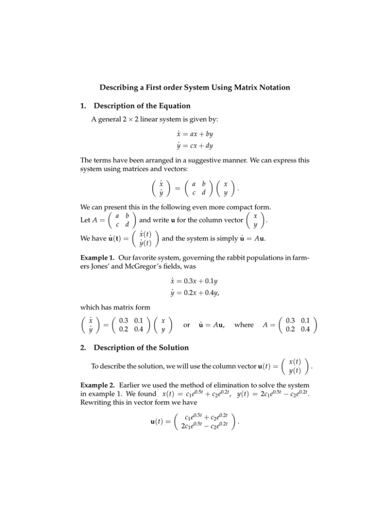
Describing a First order System Using Matrix Notation
1. Description of the Equation
A general 2 × 2 linear system is given by:
.
x = ax + by
.
y = cx + dy
The terms have been arranged in a suggestive manner. We can express this
system using matrices and vectors:
�
�� �
� . �
x
a b
x
.
=
.
c d
y
y
We can present
this
�
� in the following even more compact
� form.
�
a b
x
Let A =
and write u for the column vector
.
c d
y
� .
�
.
.
x (t)
.
We have u(t) =
and the system is simply u = Au.
y(t)
Example 1. Our favorite system, governing the rabbit populations in farm­
ers Jones’ and McGregor’s fields, was
.
x = 0.3x + 0.1y
.
y = 0.2x + 0.4y,
which has matrix form
� . � �
�� �
x
0.3 0.1
x
. =
0.2 0.4
y
y
or
.
u = Au,
�
where
A=
�
0.3 0.1
0.2 0.4
2. Description of the Solution
�
To describe the solution, we will use the column vector u(t) =
x (t)
y(t)
�
Example 2. Earlier we used the method of elimination to solve the system
in example 1. We found x (t) = c1 e0.5t + c2 e0.2t , y(t) = 2c1 e0.5t − c2 e0.2t .
Rewriting this in vector form we have
�
�
c1 e0.5t + c2 e0.2t
u(t) =
.
2c1 e0.5t − c2 e0.2t
.
Describing a First order System Using Matrix Notation
OCW 18.03SC
We can rewrite this as
u ( t ) = c1 e
0.5t
�
1
2
�
+ c2 e
0.2t
�
1
−1
�
,
which is a clearer way of presenting it. Let
� �
�
�
1
1
.5t
.2t
u1 ( t ) = e
and u2 (t) = e
.
2
−1
The column vectors u1 (t) and u2 (t) are both solutions. Since they both
involve only one form of exponential, they are sometimes known as basic
independent solutions, or normal modes. The general solution is a linear
combination of them. We will learn much more about normal modes in the
sessions on matrix methods and the phase portrait.
Remark. As with linear second order ODE’s in unit 2, the general solution
to to a 2 linear system should always consist of linear combinations of two
truly different solutions. It is not necessary , but usually our techniques
will make these two solutions the normal modes.
3. Geometry of the Solutions
Suppose you want to plot a solution u(t). As time increases, it traces a
curve in the xy-plane.
Example. The solution u1 (t) traces a ray that passes through (1, 2) at t = 0
and move off towards infinity in a straight line, with exponential speed.
There is another ray through (1, −1), corresponding to the solution u2 (t).
(This is tricky: the exponential in the formula for u1 might make you think
the trajectory is curved. However, if you look carefully at the formula you
will see u1 (t) is always a multiple of the vector (1, 2)T .)
The applet Linear phase portrait: matrix entries will allow us to visualise
this nicely, and get a feel for other sorts of trajectories. Later in this session
you will look at this applet.
2
MIT OpenCourseWare
http://ocw.mit.edu
18.03SC Differential Equations��
Fall 2011 ��
For information about citing these materials or our Terms of Use, visit: http://ocw.mit.edu/terms.