Light Scattering θ
advertisement
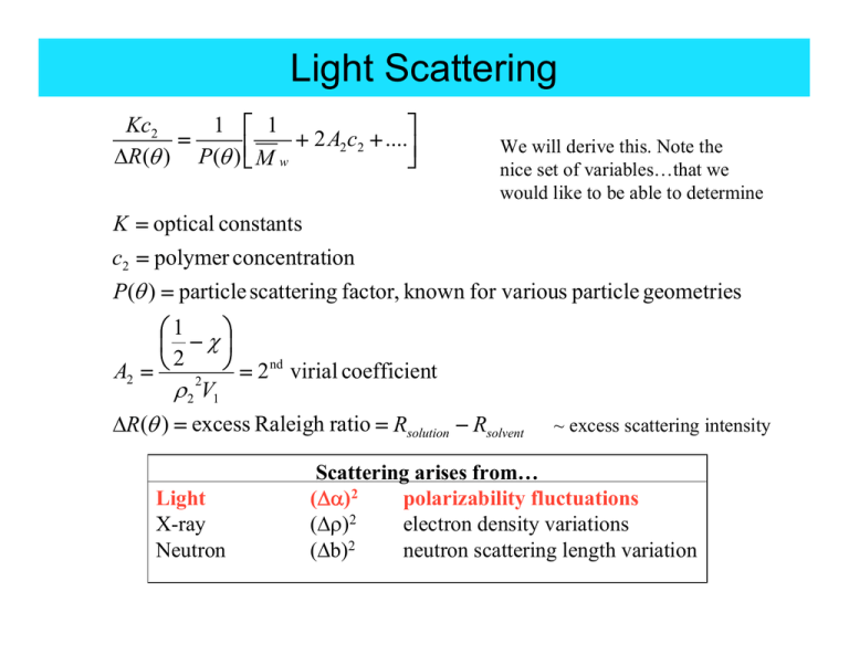
Light Scattering
1 ⎡ 1
Kc2
⎤
2
....
=
+
+
A
c
2 2
⎥⎦
ΔR(θ ) P(θ ) ⎢⎣ M w
We will derive this. Note the
nice set of variables…that we
would like to be able to determine
K = optical constants
c2 = polymer concentration
P(θ ) = particle scattering factor, known for various particle geometries
⎞
⎛1
⎜ −χ⎟
2
A2 = ⎝ 2 ⎠ = 2 nd virial coefficient
ρ 2 V1
ΔR(θ ) = excess Raleigh ratio = Rsolution − Rsolvent
Light
X-ray
Neutron
~ excess scattering intensity
Scattering arises from…
(Δα)2
polarizability fluctuations
(Δρ)2
electron density variations
(Δb)2
neutron scattering length variation
Scattering arises from Density Fluctuations
A dilute gas in vacuum
• Consider small particles:
– (situation:~ point scatterers)
dp << λradiation
Particles
dp
Incident radiation
λ
• Scattered Intensity at scattering angle θ to a detector r
away from sample:
I 8π (1+ cos θ )
α = polarizability of molecule
Iθ =
α
I0 = incident beam intensity
λr
• For N particles in total volume V (assume dilute, so no
4
2
0
2
4
2
coherent scattering)
N
Iθ = Iθ
V
'
⎛N⎞
ε = 1 + 4 π⎜ ⎟ α
⎝V⎠
ε = dielectric constant
ε = n2, ε(ω) = frequency dependent
Fundamental relationship:
index of refraction
polarizability
N
n = 1+ 4π α
V
Can approximate
n gas
dn
≅ 1+
c
dc
dn
= refractive index increment
dc
c = conc. of particles per unit volume
2
⎛ dn ⎞
⎛ dn ⎞
n = ⎜1 +
c ⎟ ≅ 1 + 2⎜ ⎟ c + . . .
⎝ dc ⎠
⎝ dc ⎠
1 (dn / dc) c
Solving gives
α=
2 π (N /V )
the polarizability
2
gas
So by analogy for a polymer-solvent solution:
dn
n ≅ n0 +
c2
dc 2
n 2 ≅ n 02 + 2 n 0
dn
c2
dc 2
Rayleigh and the Molecular Weight of Gases
2
2
π
1+
cos
θ ) ⎛ (dn / dc) c ⎞
8
⎛
⎞
N
(
'
Iθ = ⎜ ⎟
⎜
⎟
⎝V ⎠
λ4 r 2
⎝ 2π (N /V ) ⎠
simplifying
2
2
2
2
π
1+
cos
θ
I
⎛
⎞
dn
(
)
2
Iθ' = 0 4 2
⎜ ⎟c
λ r (N /V ) ⎝ dc ⎠
2
and since
N
c
=
V M / N AV
This expression contains several parameters dependent on scattering geometry, so we define
Iθ'
R=
I 0 (1+ cos 2 θ )/r 2
Rayleigh Ratio, R as
2
which equals
⎛ dn ⎞
2π 2 ⎜ ⎟ M c
⎝ dc ⎠
R=
λ4 N AV
Or just
Where K is a lumped optical constant
⎛ dn ⎞
2π 2 ⎜ ⎟
⎝ dc ⎠
K≡
λ4 N AV
2
R = K•M•c
Note, for polymer-solvent solution:
⎛
⎞
2 dn
2
2π n 0 ⎜
⎟
dc
⎝ 2⎠
K≡
λ4 N AV
Rayleigh measured the molecular weight of gas molecules
using light scattering!
2
Scattering from Fluctuations II
A dilute “gas” of polymer chains in solution
polymer coil (solute)
Debye: Re-identify fluctuations as
chains in a solvent and extend
Rayleigh’s idea to polymers in solution
pure
solvent
solvent
Incident radiation
λ
dp
coil/solvent
Vsolution
Now for polymer coils:
λ ~ dp
Recognize 4 features in a binary component system:
1.
Each cell has on average, the same number of solvent molecules
but there are variations. Fluctuations in solvent density will give rise
to some (weak) scattering (subtract off pure solvent scattering).
2.
Fluctuations in the number of solute molecules (chains) will give rise
to significant scattering
3.
Fluctuations in the concentration of solute create osmotic forces
4.
Polymer chains are large and cannot treat them as point scatterers
P(θ) ≠1
The Features of Excess Scattering
• Feature 1.
Define ΔR = Rsolution –Rpure solvent = “Excess Rayleigh Ratio”
• Feature 2.
Remaining scattering arises from fluctuations in solute concentration
2
2
2
2
⎛
⎞
dn
I
2
π
1+
cos
θ
(
)⎛⎜ dn ⎟⎞ c 2
⎟⎟ and (δc 2 )2
ΔR depends on ⎜⎜
Iθ' = 0 4 2
⎝ dc 2 ⎠
λ r (N /V ) ⎝ dc ⎠
Einstein-Smoluchowski mean squared concentration fluctuation per unit vol.
(δc2 ) =
2
RTc2
δVN AV (∂π /∂c2 )
• Feature 3.
A local osmotic pressure will arise due to local concentration differences, this
effect acts to suppress solute concentration fluctuations. Note in the gas-vacuum
system, such an effect is not present.
⎡
⎤
1
−
χ
)
(
⎢1
⎥
π
2
= RT⎢ +
c 2 + L⎥
2
V1ρ 2
c2
⎥
⎢M
⎦
⎣
∂π
⎡1
⎤
= RT ⎢ + 2A 2c 2 + L⎥
∂c 2
⎣M
⎦
Feature 3 cont’d
2
R solution − R solvent =
ΔR
2 2 ⎛⎜ dn ⎞⎟
c2
2π n 0 ⎜
⎟
⎝ dc 2 ⎠
⎤
⎡1
λ4 N AV ⎢ + 2A 2c 2 + L⎥
⎦
⎣M
Polymer in solution
Gas in vacuum
⎡
⎤
⎢
⎥
1
⎥
ΔR = Kc 2 ⎢
⎢⎛⎜ 1 + 2A c + L⎞⎟⎥
2 2
⎢⎣⎝ M
⎠⎥⎦
⎛ dn ⎞
2π 2 ⎜ ⎟ M c
⎝ dc ⎠
R=
λ4 N AV
2
similar to the Rayleigh scattering for gases but with a new term depending A2
Scattering from Polymer Solutions
• Feature 4.
Polymer chains are large and can not be assumed
as point scatterers for visible light
• λ ~ 6,328Å He-Ne laser
1001000Å
• Coil size ~ typically 100-1000 Å
depending on molecular weight of polymer
Therefore need to consider self-interference
of monomers in polymer coil on scattered intensity
• Therefore P(θ) term is important
Scattering of Polymer Solutions
Introduce finite size chain scattering factor P(θ)
ΔR = Kc2
1
⎛ 1
⎞
+ 2A2 c2 +L⎟
⎜
⎠
⎝M w
2
For a Gaussian coil P (θ ) ≡ 2 u −1+ e−u
u
(
where
)
P(θ )
(Debye, 1939)
2
⎡ 4 π n 0 ⎛ θ ⎞⎤
2
u =⎢
sin⎜ ⎟⎥ Rg
⎝ 2 ⎠⎦
⎣ λ
q = scattering vector,
u = q 2 Rg
2
In the limit of very small θ,
P(θ => 0) = 1
Useful approximation for small, nonzero θ
P (θ )
1
u
u
≈ 1− and
≈ 1+
for u1/ 2 << 1
3
P (θ )
3
Scattering in a Polymer-Solvent System
• In general, P(θ) ≠ 1, c2 ≠ 0, A2 ≠ 0
therefore rewrite excess Rayleigh ratio as
Kc2 ⎡ 1
⎤⎡ u ⎤
= ⎢ + 2A 2c 2 + L⎥ ⎢1 + ⎥
ΔR ⎣ M
⎦⎣ 3 ⎦
u = q 2 Rg
2
⎤⎡ 16π 2 n 02 2 ⎛ θ ⎞ 2 ⎤
Kc 2 ⎡ 1
= ⎢ + 2A2c 2 + L⎥⎢1+
sin ⎜ ⎟ Rg ⎥
2
⎦⎣
⎝2⎠
ΔR ⎣ M
3λ
⎦
Equation is valid for dilute solutions and scattering angles θ such that
u1/ 2 << 1
Next: how to plot scattered intensity vs. c2 and versus q2 to extract M and A2
Zimm Plot – Analysis of Light Scattering Data
Light Scattering Experiment
qo
~
Sample
q
Detector
~
Collect Scattered Intensity at typically 8 angles:
θ = 30°, 37.5°, 40°, 60°, 75°, 90°, 105°, 120°
Measure ΔR typically for 5 solute concentrations:
c2 , c2 , c2 , c2 , c2
1
2
3
4
5
Scattering Measurements:
1.
Pure (no dust!) solvent
Rsolvent
2.
Polymer solutions [c2,i , I(θi)] Rpolymer
3.
Construct Zimm Plot
Note:
Kc2
ΔRθ
ΔR = Rpolymer-Rsolvent
is a function of 2 variables, c2 and θ.
Zimm’s cool idea was to plot y(p,q) vs (p+q) to separate out
dependence on each variable: called Zimm plot
Construction of a Zimm Plot
The Master Equation:
⎛
2 2
2θ
16
π
n
sin
0
⎞⎜
Kc 2 ⎛ 1
2 R2
=⎜
+ 2 A2 c 2 + ...⎟⎜1+
g
⎠⎜
ΔR ⎝ M w
3 λ2
⎝
do double extrapolation:
θ → 0o
c2 → 0
A2 & M w
<Rg2> & M w
θ fixed for a set of concentrations
conc.
Kc2
ΔR(θi , ci )
Mole/gram
dilute
an g
small
angle
e
g
r
a
l
c fixed for a set of angles
2
le
Units
sin2(θ/2) + k c2
⎞
⎟
⎟
⎟
⎠
dimensionless axis
Zimm Plot
Sample Data Set
θ
Kc2
ΔR (θ i , ci )
c2
g/cm
30o
37.5o
45o
60o
75o
90o
105o
120o
135o
142.5o
150o
2 x 10⁻³
3.18
3.26
3.25
3.45
3.56
3.72
3.78
4.01
4.16
4.21
4.22
1.5 x 10⁻³
2.73
2.76
2.81
2.94
3.08
3.27
3.4
3.57
3.72
3.75
3.78
1 x 10⁻³
2.29
2.33
2.37
2.53
2.66
2.85
2.96
3.12
3.29
3.38
3.37
0.75 x 10⁻³
2.10
2.14
2.17
2.32
2.47
2.64
2.79
2.93
3.10
3.21
3.2
0.5 x 10⁻³
1.92
1.95
1.98
2.16
2.33
2.51
2.66
2.79
2.96
3.11
3.12
3
2
⎛
⎞
dn
2
2π 2 n 0 ⎜ ⎟
⎝ dc ⎠
K=
λ4 N AV
n 0 = 1.5014
dn = 0.106 cm 3 g−1
dc
For c2 = 0.002,
θ = 30
Kc2
= 3.18
ΔR(θ i , ci )
λ = 5.461x10⁻⁵ cm
N AV = 6.02 x10⁻²³ mole−1
Plotting the Data
“vertical” data set
θ=30˚
c2 varies (decreases)
Extrapolating to zero concentration
( .267, 3.18)
“horizontal” data sets
θ variable
c2=2x10⁻³
Kc2
ΔRθ
Image removed due to copyright restrictions.
Please see, for example,
http://web.umr.edu/~WLF/MW/orangeline.gif, from
http://web.umr.edu/~WLF/MW/Zimm.html
These points are determined
by extrapolating the equations
of each regression line
Plot typical data point :
θ = 30°,c2 = 2 ×10⁻³ g / cm 3
y-axis:
Kc2
= 3.18
ΔRθ
x-axis:
⎛ 30° ⎞
−3
sin 2 ⎜
⎟ + k(2×10 )
⎝ 2 ⎠
= 0.067 +100(2×10 −3 ) = 0.267
Pick constant to “spread” the plot
x = 0.067
Plotting the data cont’d
Extrapolating to zero scattering angle…
(.267, 3.18)
100c2
Image removed due to copyright restrictions.
Please see, for example,
http://web.umr.edu/~WLF/MW/yellowline.gif, from
http://web.umr.edu/~WLF/MW/Zimm.html
Extrapolate the extrapolated data to obtain:
Mw , A2
Kc2
ΔRθ
A
2
Image removed due to copyright restrictions.
Please see, for example,
http://web.umr.edu/~WLF/MW/first.gif, from
http://web.umr.edu/~WLF/MW/Zimm.html
Rg
2
Rg
2
A2, ⟨Rg2⟩ and
An example:
Mw
Note: units on y-axis are mole/g. The x-axis is dimensionless.
Kc2
R0
4.0
0
) ( 1+
<s2>z )
2
Kc
-1
0.1375
3.0
6
mole g
1
+ 2A2c2+
Mw
The intercept occurs at a y-value ( R2) of 1.36 x 10⁻⁶ mole/g. Hence, Mw =
0
7.35 x 10⁵ g/mole.
Now, consider the c2= 0 line. Where c2 = 0,
θ = 0 line
Kc2
1.25
R0
=
1
( 1+
Mw
0
< s2>z )
0
KC2/DR x 10
=(
c2= 0 line
2.0
1.0
slope =
0.55
0
0.4315
θ
100c2 + Sin2
2
0.5
<s2>z
1
(
Mw
Measure the slope of the c2 = 0 line.
1.0
y
slope =
=
x
)
Mw
From intercept,
M w = 735,000 g/mol
5.5 x 10⁻⁷mole/g
0.4375
= 1.26 x 10⁻⁶ mole/g
<s2>z =
=
w
3( 1.26 x 10⁻⁶ mole/g ) (7.35 x 10⁵g/mole)(5.461 x 10-5)2
16 2(1.5014)2
= 2.33 x 10⁻¹¹cm2
Figure by MIT OCW.
getting A2, ⟨Rg2⟩ and M w
(i)
r
2
<=r62 s>2
2
= 6 < Rg >
= 6 (2.33 x 10⁻¹¹ cm2)
= 1.40 x 10⁻¹⁰ cm2
r
2 1/ 2
=
1.182x10⁻⁵
cm = 1,182 A
Pretty big
molecules!
(ii) Now consider the θ = 0 line. At θ = 0 (neglecting higher order c2 terms)
Kc 2
1
=
+ 2 A2 c2
ΔR θ M w
slope = 2 A2
The density of polystyrene (ρ2) is 1.05g/cm3. The molar volume of benzene
V1 = MW/ρ1. The molecular weight of benzene is 78.11 g/mole and its
density is 0.8787g/cm3 (from CRC Handbook of Chemistry and Physics).
from the Zimm plot
3
1.25 x10⁻⁶ mole /g
−4 mole ⋅cm
= 9.09x10
= 2 A2
slope =
g2
0.1375 x10⁻² g /cm 3
A 2 = 4.55x10
−4
mole ⋅ cm 3
g2
A2, ⟨Rg2⟩ and M w
(ii) The relationship between A2 and χ is given by:
χ=
1
− A 2 V1 ρ 22
2
Substituting the values,
3
⎞
1 ⎛
−4 mole cm
χ = − ⎜ 4.55x10
⎟
g2
2 ⎝
⎠
⎛ 78.11g /mole ⎞
3 2
1.05
g
/cm
)
⎜
3 ⎟ (
0.8787
g
/cm
⎝
⎠
χ = 0.455
(So, of course, the polymer solution used for light scattering
will be a single phase since χ < 1/2
for miscibility of solvent and polymer).
Noncrystalline Materials
• The structure of noncrystalline materials (i.e. polymer
glasses, amorphous polymer melts) is characterized
by short range order (SRO)
• SRO – develops due to excluded volume and locally
dense packing (glasses ~ are only 10% less dense
than crystals)
• Pair distribution function g(r) is a dimensionless
function used to quantify SRO. In polymers SRO is
primarily due to covalent intra-molecular bonds and
neighboring intermolecular packing.
• Properties of noncrystalline polymers are heavily
influenced by τ* , the characteristic relaxation time
relative to an experimental observation time, t.
liquid (melt)
t » τ*
rubbery
t ≤ τ*
τ*(T) ?
t « τ*
glassy
Structural Features of Noncrystalline Polymers
SRO in Polymers
•
C
fixed θ
φ
C
2
C1 – C2
C1 – C3
C1 – C4
3
θ
•
C
Due to covalent intra-molecular bonds
= constant
= constant
= varies
gives rise to peaks at large q
Due to chain-chain inter-chain distances ~ 5Å
Inter-chain
1
C1 – C’1 ~ 5Å
c1
,
C1
Typical X-ray signature of noncrystalline materials broad overlapping peaks from multiple distances:
I(q)
interintraq
Pair Distribution Function g(r)
1001000Å
Figure by MIT OCW.
The Pair Distribution Function g(r) addresses the distances
between the centers of mass of pairs of units. Since
glasses and liquids are isotropic, the magnitude of the
inter-unit distance is of interest.
The scalar distance rij between molecule i and molecule j is:
rij = ⏐ri - rj⏐
g(r) cont’d
•
•
•
•
rij = ⏐ri - rj⏐
Characterize the set of distances {rij} from an average unit i to every
other unit j =1 ….. N.
g(r) counts the number of units dn in a small spherical shell
sampling volume element of size dv at each distance r from a
reference unit, dv = 4πr2dr
The statistical average of these
numbers for many units chosen
as the reference is divided by the
Figure showing the pair-distribution functions for gas, liquid or glass, and
average unit density ⟨ρ⟩
monatomic crystal removed due to copyright restrictions.
See Figure 2.5 in Allen, S. M., and E.L. Thomas. The Structure of Materials.
New York, NY: J. Wiley & Sons, 1999.
1 dn (r , r + dr )
g (r ) =
ρ dv (r , r + dr )
Features of g(r) in Glasses & Liquids
At several unit diameters,
the average number of units/vol.
becomes constant
g(r)
1.0
ξ
0
2Ro
r
Figure by MIT OpenCourseWare.
• Due to excluded volume, g(r) = 0 for distances less than 2Ro
• Liquids and glasses are strongly correlated at the shortest
distance between 2 units, the maximum occurs at
slightly > 2Ro, this largest peak is the average distance
to the first shell to the nearest-neighbor unit.
C1 C2
C1 C2
g(r)intra
C3
g(r)inter
Superposed
correlations
