6.895 Essential Coding Theory
October 20, 2004
Lecture 11
Lecturer: Madhu Sudan
1
Scribe: Anastasios Sidiropoulos
Overview
This lecture is focused in comparisons of the following properties/parameters of a code:
• List decoding, vs distance.
• Distance, vs rate.
• List decoding, vs rate.
2
The Plotkin’s Bound
Recall that for two binary strings x, y � {0, 1}n, we denote by �(x, y) the number of positions that x
and y differ.
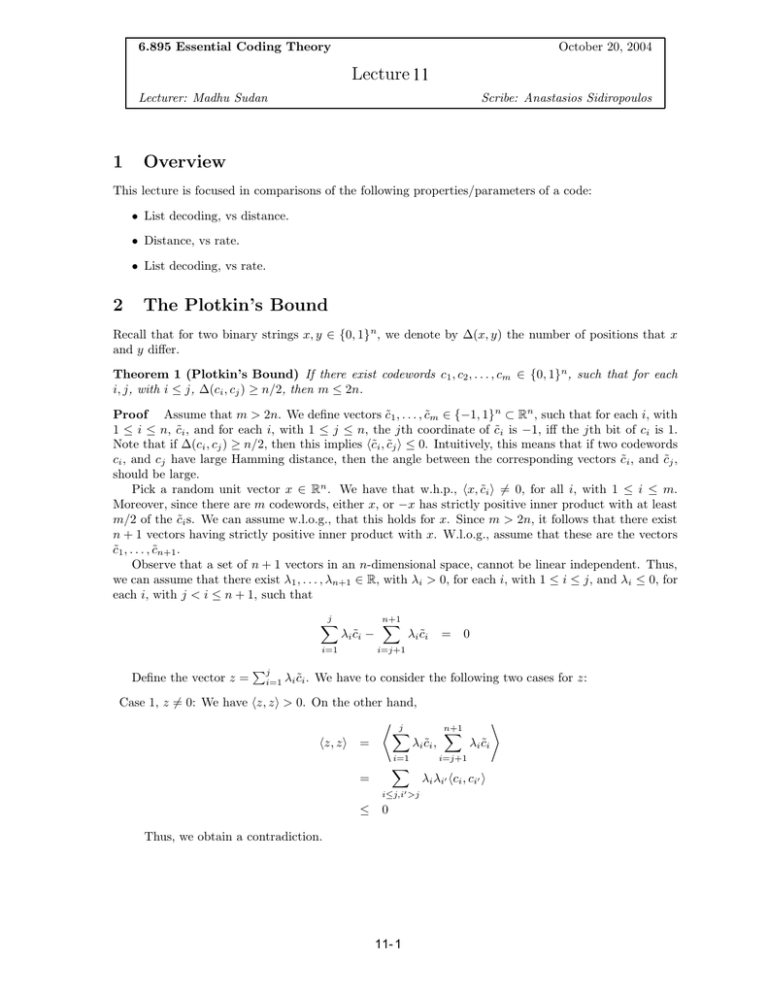
Theorem 1 (Plotkin’s Bound) If there exist codewords c1 , c2 , . . . , cm � {0, 1}n, such that for each
i, j, with i � j, �(ci , cj ) � n/2, then m � 2n.
Proof Assume that m > 2n. We define vectors c̃1 , . . . , c̃m � {−1, 1}n ≈ Rn , such that for each i, with
1 � i � n, c˜i , and for each i, with 1 � j � n, the jth coordinate of c˜i is −1, iff the jth bit of ci is 1.
Note that if �(ci , cj ) � n/2, then this implies →c̃i , c̃j ⊂ � 0. Intuitively, this means that if two codewords
ci , and cj have large Hamming distance, then the angle between the corresponding vectors c˜i , and c˜j ,
should be large.
Pick a random unit vector x � Rn . We have that w.h.p., →x, c̃i ⊂ =
√ 0, for all i, with 1 � i � m.
Moreover, since there are m codewords, either x, or −x has strictly positive inner product with at least
m/2 of the c̃i s. We can assume w.l.o.g., that this holds for x. Since m > 2n, it follows that there exist
n + 1 vectors having strictly positive inner product with x. W.l.o.g., assume that these are the vectors
c̃1 , . . . , c̃n+1 .
Observe that a set of n + 1 vectors in an n-dimensional space, cannot be linear independent. Thus,
we can assume that there exist �1 , . . . , �n+1 � R, with �i > 0, for each i, with 1 � i � j, and �i � 0, for
each i, with j < i � n + 1, such that
j
�
i=1
Define the vector z =
�j
i=1
�i c̃i −
n+1
�
�i c̃i
= 0
i=j+1
�i c̃i . We have to consider the following two cases for z:
Case 1, z √= 0: We have →z, z ⊂ > 0. On the other hand,
�
� j
n+1
�
�
→z, z ⊂ =
�i c̃i ,
�i c̃i
=
i=1
i=j+1
�
� i � i � →c i , c i � ⊂
i�j,i� >j
� 0
Thus, we obtain a contradiction.
11- 1
Case 2, z = 0: We have
j
�
�i c̃i
= 0,
i=1
and thus
�
→z, x⊂ =
j
�
�i c̃i , x
i=1
j
�
=
i=1
�
�i →c̃i , x⊂
> 0
The last inequality follows from the fact that �i > 0, for 1 � i � j, and that →c̃i , x⊂ > 0. This
however is a contradiction, since z = 0, which implies that →z, x⊂ = 0.
3
The Johnson’s Bound
�
�
�
�
(1
−
λ)n
-code,
Theorem 2 (Johnson’s Bound) For any λ, with 0 < λ < 1, if C is a n, ?, q−1
q
q
�
�
≥
(1 − λ)n errors, with lists of size (q − 1)n.
then C corrects less than q−1
q
We will give a proof of Theorem 2, for the special case of q = 2.
Proof We will prove the contrapositive. That is, we assume that there exist r, c 1 , . . . , cm � {0, 1}n,
such that for each i, with 1 � i � m,
�(r, ci )
�
1−�
n,
2
�(ci , cj )
�
1−λ
n.
2
and for each i √= j,
Define vectors r,
˜ c˜1 , . . . , c̃m � {0, 1}n ≈ Rn , as in the proof of Theorem 1. We have that for each i,
with 1 � i � m,
→r,
˜ c˜i ⊂
� � n,
→c̃i , c̃j ⊂
� λn.
and for each i √= j,
≥
We want to show that is � > e, then m � n.
We have that the projection of each c˜i into r is “large”, and that the angle between each pair of c˜i ,
c̃j is also “large”. Intuitively, the main idea of the proof is that these two properties cannot be satisfied
simultaneously, if the number of the vectors c̃i is too large. We will verify this argument by considering
the vectors c̃i − �r, for carefully chosen �, and show that the angle between each pair of such vectors is
at least 90≤ . Thus, we will obtain a bound on the number of such vectors.
11-2
Formally, we have
→ci − �r, cj − �⊂
By setting � =
≥
= →ci , cj ⊂ − �→ci , r⊂ − �→cj , r⊂ + �2 →r, r⊂
� (λ − 2�� + �2 )n
λ, we obtain that the inner product between each pair of vectors c˜i − �r, and c˜j − �r is
≥ ≥
2 λ( λ − � )n
≥
Thus, for any � < λ, the inner product is negative, and the assertion follows by applying the Plotkin’s
Bound.
We note that for the case q > 2, the proof of Theorem 2 becomes more technical. More specifically,
one needs to map each bit of a codeword ci , into more than one coordinates of the corresponding vector
c̃i . For example, if we have codewords in {0, 1, 2}n, we can map each symbol of a vector in R, such that
the angle between each vector is at lest 90≤ .
Relating R with �
4
4.1
Improving the Singleton Bound
Lemma 3 If there exists a (n, k, d)2 -code, then there also exists a (2d, k + 2d − n, d)2 -code.
Proof Let C be a (n, k, d)2 -code. C contains 2k codewords, of length n. Thus, if we project each
codeword into the first n − 2d coordinates, there are at least 2k+2d−n codewords, that are mapped into
the same string. Since all these 2k+2d−n codewords have the same prefix of length n − 2d, and since
their distance is at least d, it follows that their pairwise distance in the last 2d bits should be at least d.
Thus, the suffixes of these codewords form a (2d, k + 2d − n, d)2 code.
It follows by Lemma 3 that for any (n, k, d)2 -code, with k + 2d − n � log 4d, we have
R + 2τ − 1 � 0.
4.2
The Elias-Bassalygo Bound
The main argument in the proof of the Hamming bound is that if we have k non-intersecting balls of
n
n
radius d−1
/ 2, in {0, 1} , then the sum of their volumes cannot exceed 2 . We will show how to extend
this idea in the case of intersecting balls, by bounding the overlap.
n
Assume that we have a binary code of distance 1−�
2 . For each codeword c � {0, 1} , we consider the
�
1− �
n
ball in {0, 1} of radius 2 around c. We have
�
≥ �
1− λ
2k Vol n,
n
� n2n ,
2
and thus
2Rn 2
H
“
� ”
1− �
n
2
� 2n+o(n) .
This implies
R+H
So, if τ =
1−�
2 ,
then R + H
�1
2
−
1
2
�
≥ �
1− λ
2
≥
1 − 2τ � 1.
11- 3
� 1
4.3
The Case � � 0
An interesting question is what are the best possible codes, when τ ∈ 0. The Hamming bound gives
� �
τ
R � 1−H
2
1
1
≤ 1 − (1 + o(1))τ log2 .
2
τ
On the other hand, we know that there exist codes satisfying
R
4.4
1
� 1 − (1 + o(1))τ log2 .
τ
The Case � � 1/2
Another interesting question is what is the best possible value for R, in the case where τ = 1−�
2 , with
λ ∈ 0. The Plotkin bound gives R � 2λ. Also, the EB-bound gives R = O(λ).
On the positive side, we can show (even for the case of random codes), that there exist codes with
R = �(λ2 ).
˜ 2 ) (also known as MRRW-bound,
We also note that the Linear-Programming bound gives R = O(λ
or JPL-bound).
5
Relating R with p
We would like to know what is the best possible values for R, and p, such that for infinitely many n, we
have (n, Rn, ?)2 -codes, that are (pn, n)-error-correcting.
The Shannon bound gives
R
� 1 − H2 (p)
We will next prove that this bound is tight.
Lemma 4 There exist codes, satisfying R � 1 − H2 (p).
Before we state the proof, we note that the same result can be obtained by using random codes in
{0, 1}n, but the proof is rather technical.
Proof We will show that there exists a linear code of rate R, that is (pn, n + 1)-error-correcting. We
begin with an empty basis for the code, and we repeatedly increase the basis, by greedily adding one
base-vector at a time.
More specifically, assume that we have already added the vectors b1 , b2 , . . . , bk � {0, 1}n in the basis.
Let Ci = span(b1 , . . . , bi }. We pick bi+1 , so as to minimize the value �i+1 , where for each i, the value
�i is given by the following potential function:
�
�
�i = E 2|B(x,pn)�Ci ,
where the expectation is taken over the random choices of x, when x is distributed uniformly in {0, 1} n.
We have
E[�i+1 ] � �2i
Thus, we can conclude that there exist base vectors b1 , . . . , bk , such that
�k
� �02
11-4
k
Note that
�0
= 1+
To be continued in the next lecture . . .
11- 5
Vol(n, pn)
2n