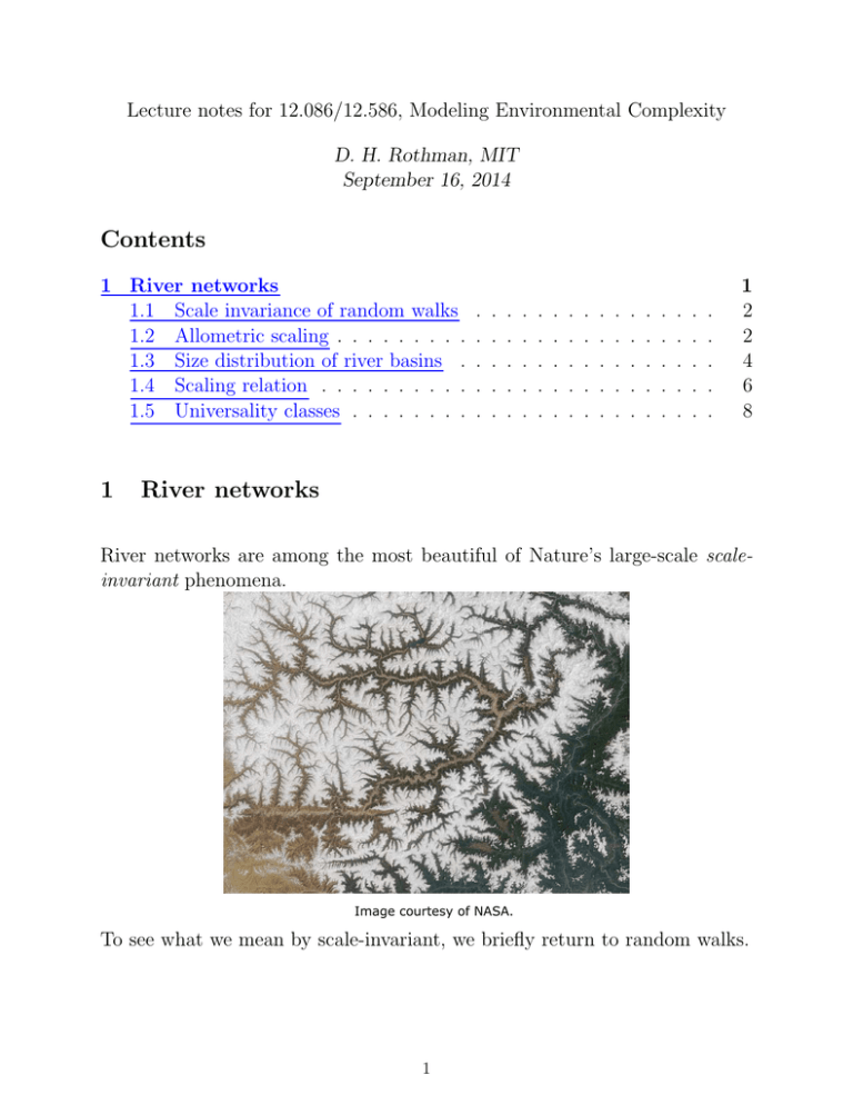
Lecture notes for 12.086/12.586, Modeling Environmental Complexity
D. H. Rothman, MIT
September 16, 2014
Contents
1 River networks
1.1 Scale invariance of random walks
1.2 Allometric scaling . . . . . . . . .
1.3 Size distribution of river basins .
1.4 Scaling relation . . . . . . . . . .
1.5 Universality classes . . . . . . . .
1
.
.
.
.
.
.
.
.
.
.
.
.
.
.
.
.
.
.
.
.
.
.
.
.
.
.
.
.
.
.
.
.
.
.
.
.
.
.
.
.
.
.
.
.
.
.
.
.
.
.
.
.
.
.
.
.
.
.
.
.
.
.
.
.
.
.
.
.
.
.
.
.
.
.
.
.
.
.
.
.
1
2
2
4
6
8
River networks
River networks are among the most beautiful of Nature’s large-scale scaleinvariant phenomena.
Image courtesy of NASA.
To see what we mean by scale-invariant, we briefly return to random walks.
1
1.1
Scale invariance of random walks
Define the rms excursion r = hx2 (t)i1/2 . We have previously shown that
r ∝ t1/2 .
Now rescale time t → bt and note that
r(t) = b−1/2 r(bt).
This simple manipulation yields a remarkable observation: the statistics of
the random walk are unchanged by the simultaneous rescaling
x → b1/2 x,
t → bt.
This means that the random walk is statistically equivalent at all scales, e.g.
Here b = 1/5 and the inset is “blown up”
√ by stretching the horizontal axis
by a factor of 5 and the vertical axis by 5.
[Another example: go to any financial website that provides graphs of market
fluctuations at a time scale of your choosing (days, weeks, months, years).
Note that aside from long-term trends, all graphs look alike!]
Although we present the random walk as an example of scale-invariance, note
that space and time do not scale in the same way.
Such scaling is called self-affine, but for now it suffices to simply note the
statistical equivalence at different scales.
1.2
Allometric scaling
River basins exhibit a similar phenomenon: they too have statistically similar
shapes at all scales, but their dimensions scale differently.
2
We refer to the two lengths as Lk and L⊥ :
The area a is
a ∝ L k L⊥ .
Measurements made from maps typically show
L⊥ ∝ LkH ,
1/2 . H . 1
and therefore
a ∝ L1+H
k
The case H = 1 in (a) yields geometric similarity or self-similarity: no matter
what the size of a, all basins “look alike.”
The case H 6= 1 in (b) is called allometric scaling (as opposed to “isometric”):
dimensions grow at different rates.
Specifically,
1 H−1
1−H
L⊥
H−1
∝ Lk ∝ a 1+H
= a− 1+H .
Lk
Since observed values of H fall within 0 < H < 1,
1−H
> 0.
1+H
Therefore
• large river basins tend to be long and thin; and
• small river basins tend to be short and fat.
Upon appropriate rescaling, however, they all look the same.
3
1.3
Size distribution of river basins
Suppose we stand at a point x0 chosen at random on a landscape. What is
the size of the area a that drains into it?
We could estimate a by walking uphill from x0 , always following the steepest
path. That brings us to a drainage divide, providing an estimate of Lk .
Obtaining the full area a, however, requires more work. A particularly labor
intensive method would be to create a grid of, say, 1 m, and to place a person
at each grid site above x0 . We then ask each person to follow his/her path of
steepest descent from one grid site to the next. Then if N people eventually
arrive at x0 , the drainage basin has size N m2 .
But what would a be a step to the right or left?
More generally, what is the probability distribution Pa (a) of drainage areas?
To answer this question we create a model of a landscape made of random
bumps. The bumps are smooth on a small scale but otherwise independently
chosen from some well-behaved distribution like a Gaussian.
We then tilt the landscape so that all paths of steepest descent are always
directed in the direction of the tilt.
We then populate the landscape as before, and follow each path of steepest
descent. Supposing that the square grid is oriented 45◦ to the tilt direction,
each step down will also be a step to the left or right, and the coalescence of
the various paths will look like this:
4
If we then trace out any basin, we find that its left and right boundaries are
particular realizations of a random walk.
This is Scheidegger’s 1967 model of river networks [1].
Since for a random walk we have hx2 i1/2 ∝ t1/2 , we substitute
t → Lk ,
x → L⊥
and conclude
1/2
L⊥ ∝ Lk
⇒
3/2
a ∝ Lk .
Since our random walks are always directed toward the bottom boundary, the
length l of the longest stream in each basin scales like l ∝ Lk , and therefore
l ∝ a2/3
Real rivers exhibit a similar scaling law, called Hack’s Law [2]:
l ∝ ah ,
0.57 . h . 0.60.
The correspondence between the two suggests that our model is reasonable.
To find Pa (a), we write
φl (y) = left basin boundary
φr (y) = right basin boundary
and assume that they both start at y = 0. Note that the difference
φ(y) = φl (y) − φr (y)
is itself a random walk that not only begins at y = 0 but also ends at y = 0.
5
We ask a precise question: What is the probability that φ(y) returns to its
initial position for the first time after n steps?
This is the classic first-return or first-passage time of a random walk. The
answer, for large n, is [3, 4]
1
P (n) = √ n−3/2 .
2 π
Since our random walks are directed, the main stream length l ∝ n. Therefore
Pl (l) ∝ l−3/2 .
To obtain the area distribution, we recall l ∝ a2/3 and write
dl
Pa (a) = Pl l(a)
da
2/3 −3/2 −1/3
∝ (a )
a
= a−4/3 .
Real rivers exhibit
Pa (a) ∝ a−τ ,
τ = 1.43 ± 0.02,
suggesting once again that our model is reasonable.
1.4
Scaling relation
Gathering our results, we have
l ∝ ah
Pa (a) ∝ a−τ
Pl (l) ∝ l−γ
where, comparing Scheidegger’s random-walk model to real observations, we
have
Exponent Scheidegger Real world
h
2/3
0.58 ± 0.02
τ
4/3
1.43 ± 0.02
γ
3/2
1.8 ± 0.1
6
Since we are looking at areas and lengths, we expect that, whatever their real
values, the exponents h, τ , and γ should be related to each other. We find
this relation by writing
dl
Pa (a) = Pl l(a)
da
h −γ h−1
∝ (a ) a
= a−[1−h(1−γ)] ,
which yields
τ = 1 − h(1 − γ).
This is an example of a scaling relation: an algebraic relationship that gives
the explicit dependence between exponents. In this case, it says that we need
only know two exponents to obtain the third. (Further work [5,6] shows that
there is only one independent exponent.)
Our scaling relation is readily verified by substituting the value for Scheidegger’s model:
2
3
4
=1−
1−
3
3
2
As for the real world, we have
1.43 ' 1 − 0.58(1 − 1.8) = 1.46.
Overall we see that the statistical geometry of river networks—the powerlaw scaling, and the relations between the exponents—is well described by
Scheidegger’s random walks.
Note that we have said nothing about how real rivers form.
Instead we note that their tendency to aggregate (i.e., connect) as they flow
downhill is the main ingredient necessary to account for their principal geometric features after they form.
We suspect that this reflects the universal properties of random walks: i.e.,
that the mean square fluctuation in one dimension scales roughly like the
mean fluctuation in the other.
7
If this is true, it means that natural landscapes contain no particularly special
features that suggest that the typical paths of steepest descent are unlike
random walks.
That the Scheidegger model does not capture the correct values of the exponents τ , h, and γ suggests nevertheless that something important is missing.
We proceed to consider what that might be.
1.5
Universality classes
Let us consider our random-walk model as a member of a wider class of
models based on the kind of path taken by flowing water:
• (a) Non-convergent.
• (b) Directed random walks (Scheidegger).
• (c) Undirected random walks.
Now consider Hack’s law l ∝ ah .
The trivial non-convergent case (a) yields h = 1.
Directed random walks (b) yield h = 2/3.
Undirected random walks (c) yield h = 5/8 [7].
Remaining exponents are obtained from our previous scaling relation, augmented by the additional relation τ = 2 − h [5, 6].
8
Each of these cases may be considered universality classes. These classes are
delineated by qualitative conditions: here, the way in which flowing water
can aggregate. These qualitative conditions then lead to specific quantitative
predictions of exponents.
Which universality class is “correct”? One could argue that undirected random walks are the most realistic class, and that it is no surprise that their
Hack exponent, h = 5/8, is the closest to the observed h ' 0.58.
Although such reasoning may possibly be valid, it misses the main lesson:
Aggregating random walks capture the main features of river network geometry.
All the rest comes down to getting the exponents “right.” But because it is
not precisely clear what it would mean to be correct, it is both more interesting and safer to simply learn our lesson and ask if it has any applicability
elsewhere.
References
[1] Scheidegger, A. E. A stochastic model for drainage patterns into an intramontane trench. Bull. Int. Assoc. Sci. Hydrol. 12, 15–20 (1967).
[2] Hack, J. T. Studies of longitudinal stream profiles in Virginia and Maryland. U.S. Geological Survey Professional Papers 294-B, 45–97 (1957).
[3] Feller, W. An Introduction to Probability Theory and Its Applications
(John Wiley & Sons, New York, 1968).
[4] Redner, S. A Guide to First-Passage Processes (Cambridge University
Press, Cambridge, UK, 2001).
[5] Dodds, P. S. & Rothman, D. H. A unified view of scaling laws for river
networks. Phys. Rev. E. 59, 4865–4877 (1999).
[6] Dodds, P. S. & Rothman, D. H. Scaling, universality, and geomorphology.
Annu. Rev. Earth Planet. Sci. 28, 571–610 (2000).
9
[7] Manna, S. S., Dhar, D. & Majumdar, S. N. Spanning trees in two dimensions. Phys. Rev. A 46, 4471–4474 (1992).
10
MIT OpenCourseWare
http://ocw.mit.edu
12.086 / 12.586 Modeling Environmental Complexity
Fall 2014
For information about citing these materials or our Terms of Use, visit: http://ocw.mit.edu/terms.