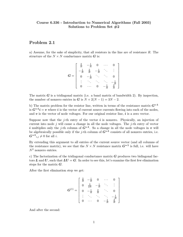
Course 6.336 ­ Introduction to Numerical Algorithms (Fall 2003)
Solutions to Problem Set #2
Problem 2.1
a) Assume, for the sake of simplicity, that all resistors in the line are of resistance R. The
structure of the N × N conductance matrix G is:
⎡
⎢
⎢
⎢
⎢
G=⎢
⎢
⎢
⎢
⎣
2
R
− R1
0
..
.
0
−
R1
0
···
..
1
.
−R
. .
..
.
.
..
..
.
.
0 − R1
2
R
− R1
..
.
···
⎤
0
.. ⎥
. ⎥
⎥
⎥
⎥
0
⎥
⎥
⎥
− R1 ⎦
2
R
The matrix G is a tridiagonal matrix (i.e. a band matrix of bandwidth 2). By inspection,
the number of nonzero entries in G is N + 2(N − 1) = 3N − 2.
b) The matrix problem for the resistor line, written in terms of the resistance matrix G�1
is G�1 i = v where i is the vector of current source currents flowing into each of the nodes,
and v is the vector of node voltages. For our original resistor line, i is a zero vector.
Suppose now that the j­th entry of the vector i is nonzero. Physically, an injection of
current into node j will cause a change in all the node voltages. The j­th entry of vector
i multiplies only the j­th column of G�1 . So a change in all the node voltages in v will
be algebraically possible only if the j­th column of G�1 consists of all nonzero entries, i.e.
G�1 i,j =
� 0 for all i.
By extending this argument to all entries of the current source vector (and all columns of
the resistance matrix), we see that the N × N resistance matrix G�1 is full, i.e. will have
N 2 nonzero entries.
c) The factorization of the tridiagonal conductance matrix G produces two bidiagonal fac­
tors L and U , such that LU = G. In order to see this, let’s examine the first few elimination
steps for the matrix G.
After the first elimination step we get:
⎡ 2
R
⎢
⎢ 0
⎢
⎢
G(1) = ⎢
⎢ 0
⎢ .
⎢ .
⎣ .
0
−
R1
0
3
2R
− R1
− R1
.
···
.
0
2
R
..
..
And after the second:
1
···
0
.
..
.
..
.
.
.
0
..
.
− R1
1
2
−R
R
⎤
⎥
⎥
⎥
⎥
⎥
⎥
⎥
⎥
⎦
⎡ 2
R
⎢
⎢ 0
⎢
⎢
⎢ 0
⎢
G(2) = ⎢ .
⎢ .
⎢ .
⎢
⎢ ..
⎣ .
0
− R1
3
2R
0
..
.
0
..
.
4
3R
− R1
..
···
.
···
···
..
.
..
.
2
R
..
···
..
.
..
.
..
.
.
1
0 −R
0
...
..
.
⎤
⎥
⎥
⎥
⎥
⎥
⎥
⎥
⎥
0 ⎥
⎥
1 ⎥
−R ⎦
2
R
Each elimination step targets only one row in the tridiagonal matrix G. In addition, the
triangular block of zeros in the upper­right corner of the matrix remains untouched. Thus
after all N − 1 elimination steps, the L matrix will feature ones on the main diagonal, and
the N − 1 multipliers on the sub­diagonal. The U matrix will also be bidiagonal, with the
pivots on the main diagonal, and −R’s on the super­diagonal. It follows that the number
of nonzero entries in L or U is thus N + (N − 1) = 2N − 1.
For N = 1000 the number of nonzero entries in G�1 is 1, 000, 000 while L and U will each
contain only 1999 nonzero entries. It is not a good idea to use the inverse of a matrix
for solving the matrix problem due to the excessive number of required multiplications
proportional to the number of nonzero entries.
d) To determine the smallest entry in the resistance matrix, let’s use the fact that an entry
rij if the resistance matrix is simply a voltage at node i caused by a unit current source
connected to node j. And we are looking for a smallest entry, i.e. the case where voltage is
minimal. You can easily figure out that we should put current source at one ends of the line
and examine the voltage at the other end of the line. In other words, the smallest element
for an N xN resistance matrix is always r1N or rN 1 ­ they are equal, since matrix inversion
preserves symmetry.
Now imagine our line with current source connected to the first node. The voltage at node
N is evidently
r1N =
1
N +1
(1)
Note, that for N xN matrix correspond to N + 1­length resistor line.
Problem 2.2
a) It is very easy to find counter­example, just remember the fomula for, say, second pivot:
a
˜22 = a22 − a21
a12
a11
(2)
Evidently, there is no guarantee that |a
˜22 | ≤ |a22 |.
b) The statement is true. For example, (2) implies that |a
˜22 |le|a22 |. Therefore we have
proven the statement for order 2. To prove the statement in general case, we need to use
2
mathematical induction. Let’s assume that we have proven our statement for the order
N − 1. Now we need to show, that for the order N of the matrix, after eliminating first row
from all subsequent rows, the resulting (N − 1)x(N − 1) submatrix:
1. will have all positive diagonal entries, no larger than original diagonal entries
2. will have negative off­diagonals
3. will be strictly diagonally dominant
4. will be tridiagonal
Thie first statement we have already shown, since all multipliers except for the M21 are
zero. Second one is also trivial. Same is the last one.
Now, let’s show that the third statement holds. Since initial matrix is strictly diagonally
dominant, we know that |a22 | > |a21 | + |a23 |, and |a11 | > |a12 |. The only thing we need
to show is that the number we substract from a22 is less than a2 1, which is also evident.
Therefore we have:
|˜
a22 | > a22 − |a21 | > |a21 | + |a23 | − |a21 | = |a
˜23 |
(3)
We have proved the statement in general case.
Problem 2.3
a) For N (y, k) = I + yeTk and given k, the matrix N structurally looks like:
k
1 ···
y1
··· 0
⎢ . .
.
⎢ ..
..
..
...
⎢
⎢
N (y, k) = ⎢ 0 · · · 1 + yk · · · 0
⎢ .
..
. . ..
⎢ .
. .
⎣ .
.
0 ···
yn
··· 1
⎡
⎤
⎥
⎥
⎥
⎥
⎥
⎥
⎥
⎦
where y = [y1 · · · yn ]T . A simple check will help you verify that N −1 is structurally similar
to N . Let
k
1 · · · w1 · · · 0
⎢ . .
⎢ ..
. . ...
...
⎢
⎢
= ⎢ 0 · · · wk · · · 0
⎢ .
.. . . ..
⎢ .
. .
⎣ .
.
0 · · · wn · · · 1
⎡
N −1
3
⎤
⎥
⎥
⎥
⎥
⎥
⎥
⎥
⎦
Furthermore, since N N −1 = I we get the following system in n unknowns:
⎧
w1 + y1 wk =
⎪
⎪
⎪
⎪
⎪
w2 + y2 wk =
⎪
⎪
⎪
⎪
⎨
... =
⎪
(1 + yk )wk =
⎪
⎪
⎪
⎪
⎪
... =
⎪
⎪
⎪
⎩
0
0
0
1
0
wn + yn wk = 0,
or equivalently N w = ek . Solving this system for w = [w1 · · · wn ]T gives a formula for
obtaining N −1 :
⎡
N −1
⎢
⎢
⎢
⎢
= ⎢
⎢
⎢
⎢
⎣
1
..
.
0
..
.
0
k
y1
· · · − (1+y
k)
.
..
.
.
.
1
· · · (1+yk )
..
.
yn
· · · − (1+y
k)
··· 0
...
··· 0
. . ..
. .
··· 1
b) Using the result in part a) we see that
N (y, k)x = ek
or equivalently
(I + yeTk )x = ek
from where we get successively
x + xk y = ek
and
y=
1
(ek − x).
xk
c) Say we wish to find the inverse of the matrix A,
⎡
⎢
⎢
⎢
A = ⎢
⎢
⎣
a11 a12
a21 a22
··· ···
··· ···
an1 a12
Let us write A as
4
· · · a1n
· · · a2n
··· ···
··· ···
· · · ann
⎤
⎥
⎥
⎥
⎥
⎥
⎦
⎤
⎥
⎥
⎥
⎥
⎥
⎥
⎥
⎥
⎦
⎡
⎤
⎢
⎢
⎢
A = ⎢ x(0)
⎢ 1
⎣
(0)
x
2
···
(0)
xn
⎥
⎥
⎥
⎥
⎥
⎦
(0)
where xj denotes the jth column of A at step 0 of our (yet­to­be derived) matrix inversion
algorithm.
In part (b) we showed how to find a matrix N such that N x = ek for a given x. Let us
notate this matrix by N (x, k) so that N (x, k)x = ek . In the first step of the algorithm we
(0)
compute N (x1 , 1) and multiply it into A, so that
⎡
(0)
N (x1 , 1)A
where
(1)
xj
⎢
⎢
⎢
=⎢
⎢
⎣
1
0
(1)
(1)
0 x2
· · · xn
0
0
(0)
⎤
⎥
⎥
⎥
⎥
⎥
⎦
(0)
= N (x1 , 1)xj
(0)
(1)
We now multiply N (x1 , 1)A by N (x2 , 2), and so forth, so that after k steps, we have
⎡
⎢
⎢
⎢
(� �1)
N (x�
, j)A
= ⎢
⎢
⎢
j=1
⎣
k
�
1 0
0 1
(k)
(k)
0 0 · · · xk+1 · · · xn
.. ..
. .
0 0
⎤
⎥
⎥
⎥
⎥
⎥
⎥
⎦
where the column vectors at step k are
(k)
xj
=
k
�
(j−1)
N (xj
(0)
, j)xj
j=1
(k−1)
It is fairly easy to convince yourself that multiplication by N (xk
, k) does not affect the
(k−1)
first k − 1 columns of the matrix, since the first k − 1 columns of both N (xk
, k) and
�k
(� �1)
, j)A are the identity vectors e. Thus,
j =1 N (x�
A−1 =
n
�
(j−1)
N (x
j
, j)
j=1
(k)
What makes the algorithm in­place is that since xj≤k = ej , we no longer have to store those
�
(j−1)
, j) is el for l > k. Thus, we can accumulate A−1
vectors. Also, column l of kj =1 N (xj
in the space occupied by the columns of A that have already been reduced to unit vectors.
5
(k−1)
Note that if at some step k, xk
[k] = 0, then this algorithm will fail. The solution is to
pivot by swapping columns in the matrix. I haven’t included code that performs pivoting,
because that is the subject of the next problem set.
Some of you noticed that this is essentially the procedure known as “Jordan elimination.”
Jordan elimination is in some sense an extension of Gaussian elimination to the extent that
at each point in the elimination the elements on previous pivotal rows are also eliminated.
The following code implements these ideas by expliciting forming all the required products.
%in-place invert a matrix A
n = size(A,1);
for i=1:n,
y = -A(:,i);
y(i) = y(i) + 1.0;
y = y / A(i,i);
for k = i+1:n;
m = A(i,k);
for j=1:n;
A(j,k) = A(j,k) + m * y(j);
end;
end;
A(:,i) = y;
A(i,i) = A(i,i) + 1.0;
for k = 1:i-1;
m = A(i,k);
for j=1:n;
A(j,k) = A(j,k) + m * y(j);
end;
end;
end;
On a Sun Sparc­10, this routine is about 500 times slower that Matlab’s builtin inv()
function.
A more efficient code would operate on the matrix by columns:
%in-place invert a matrix A; vectorized
n = size(A,1);
for i=1:n,
y = -A(:,i);
y(i) = y(i) + 1.0;
y = y / A(i,i);
for k = i+1:n;
A(:,k) = A(:,k) + A(i,k) * y;
end;
A(:,i) = y;
A(i,i) = A(i,i) + 1.0;
for k = 1:i-1;
6
A(:,k) = A(:,k) + A(i,k) * y;
end;
end;
This routine is significantly faster; it is only a factor of 10­15 slower than Matlab. Regardless
of how fast the machine is, the fact that direct matrix inversion takes O(N 3 ) operations
limits the size of the problem we can solve in a reasonable time. Matlab took roughly 2.7
seconds to invert an N = 250 matrix. In a month, it could probably do N = 25000, in a
year, about N = 50000. The first algorithm above could probably handle only N = 3000
in a month, N = 7000 in a year.
7