Algorithm paradigms
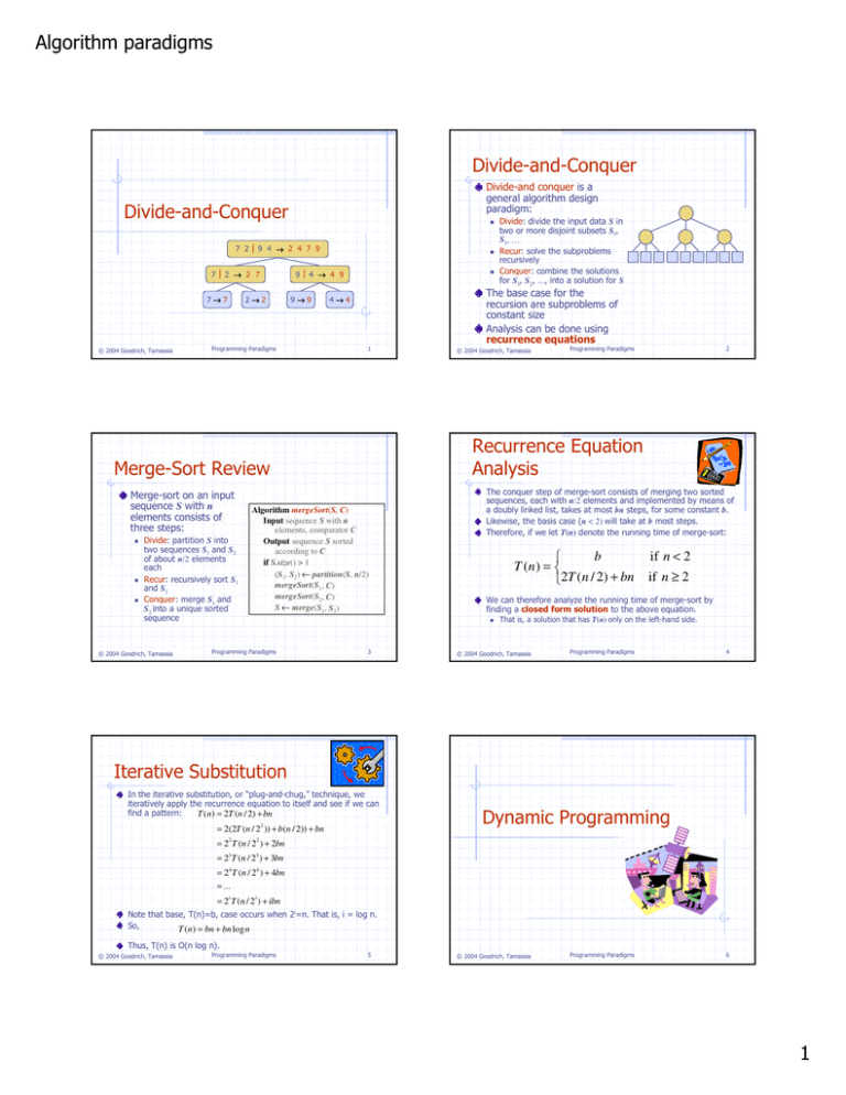
Divide-and-Conquer
Divide-and conquer is a
general algorithm design
paradigm:
Divide-and-Conquer
„
7 29 4 → 2 4 7 9
72 → 2 7
7→7
© 2004 Goodrich, Tamassia
2→2
„
94 → 4 9
9→9
Programming Paradigms
„
4→4
1
„
„
„
Divide: partition S into
two sequences S1 and S2
of about n/2 elements
each
Recur: recursively sort S1
and S2
Conquer: merge S1 and
S2 into a unique sorted
sequence
© 2004 Goodrich, Tamassia
The base case for the
recursion are subproblems of
constant size
Analysis can be done using
recurrence equations
© 2004 Goodrich, Tamassia
Algorithm mergeSort(S, C)
Input sequence S with n
elements, comparator C
Output sequence S sorted
according to C
if S.size() > 1
(S1, S2) ← partition(S, n/2)
mergeSort(S1, C)
mergeSort(S2, C)
S ← merge(S1, S2)
2
The conquer step of merge-sort consists of merging two sorted
sequences, each with n/2 elements and implemented by means of
a doubly linked list, takes at most bn steps, for some constant b.
Likewise, the basis case (n < 2) will take at b most steps.
Therefore, if we let T(n) denote the running time of merge-sort:
b

T (n ) = 
2T ( n / 2) + bn
3
if n < 2
if n ≥ 2
We can therefore analyze the running time of merge-sort by
finding a closed form solution to the above equation.
„
Programming Paradigms
Programming Paradigms
Recurrence Equation
Analysis
Merge-Sort Review
Merge-sort on an input
sequence S with n
elements consists of
three steps:
Divide: divide the input data S in
two or more disjoint subsets S1,
S2, …
Recur: solve the subproblems
recursively
Conquer: combine the solutions
for S1, S2, …, into a solution for S
That is, a solution that has T(n) only on the left-hand side.
© 2004 Goodrich, Tamassia
Programming Paradigms
4
Iterative Substitution
In the iterative substitution, or “plug-and-chug,” technique, we
iteratively apply the recurrence equation to itself and see if we can
find a pattern:
T ( n ) = 2T ( n / 2) + bn
= 2(2T ( n / 22 )) + b( n / 2)) + bn
Dynamic Programming
= 2 T ( n / 2 ) + 2bn
2
2
= 23 T ( n / 23 ) + 3bn
= 2 4 T ( n / 24 ) + 4bn
= ...
= 2i T ( n / 2i ) + ibn
Note that base, T(n)=b, case occurs when 2i=n. That is, i = log n.
So,
T ( n) = bn + bn log n
Thus, T(n) is O(n log n).
© 2004 Goodrich, Tamassia
Programming Paradigms
5
© 2004 Goodrich, Tamassia
Programming Paradigms
6
1
Algorithm paradigms
Analyzing the Binary Recursion
Fibonacci Algorithm
Computing Fibonacci Numbers
Let nk denote number of recursive calls made by
BinaryFib(k). Then
Fibonacci numbers are defined recursively:
F0 = 0
F1 = 1
Fi = Fi-1 + Fi-2
„
„
„
for i > 1.
„
As a recursive algorithm (first attempt):
„
„
Algorithm BinaryFib(k):
Input: Nonnegative integer k
Output: The kth Fibonacci number Fk
if k = 1 then
return k
else
return BinaryFib(k - 1) + BinaryFib(k - 2)
Programming Paradigms
© 2004 Goodrich, Tamassia
„
„
„
7
„
„
9
„
k
Subsequence: ACEGJIK
Subsequence: DFGHK
Not subsequence: DAGH
© 2004 Goodrich, Tamassia
Programming Paradigms
1+1+1=3
3+1+1=5
5+3+1=9
9 + 5 + 1 = 15
15 + 9 + 1 = 25
25 + 15 + 1 = 41
41 + 25 + 1 = 67.
Programming Paradigms
8
Simple subproblems: the subproblems can be
defined in terms of a few variables, such as j, k, l,
m, and so on.
Subproblem optimality: the global optimum value
can be defined in terms of optimal subproblems
Subproblem overlap: the subproblems are not
independent, but instead they overlap (hence,
should be constructed bottom-up).
© 2004 Goodrich, Tamassia
Programming Paradigms
10
Given two strings X and Y, the longest
common subsequence (LCS) problem is
to find a longest subsequence common
to both X and Y
Has applications to DNA similarity
testing (alphabet is {A,C,G,T})
Example: ABCDEFG and XZACKDFWGH
have ACDFG as a longest common
subsequence
A subsequence of a character string
x0x1x2…xn-1 is a string of the form
xi xi …xi , where ij < ij+1.
Not the same as substring!
Example String: ABCDEFGHIJK
„
=
=
=
=
=
=
=
The Longest Common
Subsequence (LCS) Problem
Subsequences (§ 12.5.1)
„
© 2004 Goodrich, Tamassia
„
Runs in O(k) time.
2
1
1
1
1
1
1
1
Applies to a problem that at first seems to
require a lot of time (possibly exponential),
provided we have:
Algorithm LinearFibonacci(k):
Input: A nonnegative integer k
Output: Pair of Fibonacci numbers (Fk, Fk-1)
if k = 1 then
return (k, 0)
else
(i, j) = LinearFibonacci(k - 1)
return (i +j, i)
1
+
+
+
+
+
+
+
The General Dynamic
Programming Technique
Use linear recursion instead:
Programming Paradigms
n0
n1
n2
n3
n4
n5
n6
Note that the value at least doubles for every other
value of nk. That is, nk > 2k/2. It is exponential!
A Better Fibonacci Algorithm
© 2004 Goodrich, Tamassia
n0 = 1
n1 = 1
n2 = n1 +
n3 = n2 +
n4 = n3 +
n5 = n4 +
n6 = n5 +
n7 = n6 +
n8 = n7 +
11
© 2004 Goodrich, Tamassia
Programming Paradigms
12
2
Algorithm paradigms
A Poor Approach to the
LCS Problem
A Dynamic-Programming
Approach to the LCS Problem
A Brute-force solution:
„
„
„
Enumerate all subsequences of X
Test which ones are also subsequences of Y
Pick the longest one.
Analysis:
„
„
If X is of length n, then it has 2n
subsequences
This is an exponential-time algorithm!
© 2004 Goodrich, Tamassia
Programming Paradigms
Define L[i,j] to be the length of the longest common
subsequence of X[0..i] and Y[0..j].
Allow for -1 as an index, so L[-1,k] = 0 and L[k,-1]=0, to
indicate that the null part of X or Y has no match with the
other.
Then we can define L[i,j] in the general case as follows:
1. If xi=yj, then L[i,j] = L[i-1,j-1] + 1 (we can add this match)
2. If xi≠yj, then L[i,j] = max{L[i-1,j], L[i,j-1]} (we have no
match here)
Case 1:
13
An LCS Algorithm
© 2004 Goodrich, Tamassia
Case 2:
Programming Paradigms
14
Visualizing the LCS Algorithm
Algorithm LCS(X,Y ):
Input: Strings X and Y with n and m elements, respectively
Output: For i = 0,…,n-1, j = 0,...,m-1, the length L[i, j] of a longest string
that is a subsequence of both the string X[0..i] = x0x1x2…xi and the
string Y [0.. j] = y0y1y2…yj
for i =1 to n-1 do
L[i,-1] = 0
for j =0 to m-1 do
L[-1,j] = 0
for i =0 to n-1 do
for j =0 to m-1 do
if xi = yj then
L[i, j] = L[i-1, j-1] + 1
else
L[i, j] = max{L[i-1, j] , L[i, j-1]}
return array L
© 2004 Goodrich, Tamassia
Programming Paradigms
15
© 2004 Goodrich, Tamassia
Programming Paradigms
16
Analysis of LCS Algorithm
We have two nested loops
„
„
„
„
The outer one iterates n times
The inner one iterates m times
A constant amount of work is done inside
each iteration of the inner loop
Thus, the total running time is O(nm)
The Greedy Method and
Text Compression
Answer is contained in L[n,m] (and the
subsequence can be recovered from the
L table).
© 2004 Goodrich, Tamassia
Programming Paradigms
17
© 2004 Goodrich, Tamassia
Programming Paradigms
18
3
Algorithm paradigms
The Greedy Method
Technique (§ 12.4.2)
Text Compression (§ 12.4)
The greedy method is a general algorithm
design paradigm, built on the following
elements:
„
„
Given a string X, efficiently encode X into a
smaller string Y
configurations: different choices, collections, or
values to find
objective function: a score assigned to
configurations, which we want to either maximize or
minimize
a globally-optimal solution can always be found by a
series of local improvements from a starting
configuration.
Programming Paradigms
© 2004 Goodrich, Tamassia
19
Encoding Tree Example
„
„
„
„
010
011
10
11
a
b
c
d
e
© 2004 Goodrich, Tamassia
a
Programming Paradigms
d
b
Given a text string X, we want to find a prefix code for the characters
of X that yields a small encoding for X
c
© 2004 Goodrich, Tamassia
„
X = abracadabra
T1 encodes X into 29 bits
T2 encodes X into 24 bits
„
„
„
T1
T2
c
d
a
21
b
c
c
d
r
5
2
1
1
2
d
1
6
2
c
23
b
2
c
© 2004 Goodrich, Tamassia
4
d
b
6
r
2
a
5
c
2
d
r
2
r
2
2
a
5
d
11
b
c
1
r
22
a
a
b
2
b
Programming Paradigms
X = abracadabra
Frequencies
a
5
a
r
© 2004 Goodrich, Tamassia
Example
Algorithm HuffmanEncoding(X)
Input string X of size n
Output optimal encoding trie for X
C ← distinctCharacters(X)
computeFrequencies(C, X)
Q ← new empty heap
for all c ∈ C
T ← new single-node tree storing c
Q.insert(getFrequency(c), T)
while Q.size() > 1
f1 ← Q.minKey()
T1 ← Q.removeMin()
f2 ← Q.minKey()
T2 ← Q.removeMin()
T ← join(T1, T2)
Q.insert(f1 + f2, T)
return Q.removeMin()
Programming Paradigms
Frequent characters should have long code-words
Rare characters should have short code-words
„
Example
e
Huffman’s Algorithm
Given a string X,
Huffman’s algorithm
construct a prefix
code the minimizes
the size of the
encoding of X
It runs in time
O(n + d log d), where
n is the size of X
and d is the number
of distinct characters
of X
A heap-based
priority queue is
used as an auxiliary
structure
20
Encoding Tree Optimization
Each external node stores a character
The code word of a character is given by the path from the root to
the external node storing the character (0 for a left child and 1 for a
right child)
00
Programming Paradigms
© 2004 Goodrich, Tamassia
A code is a mapping of each character of an alphabet to a binary
code-word
A prefix code is a binary code such that no code-word is the
prefix of another code-word
An encoding tree represents a prefix code
„
Compute frequency f(c) for each character c.
Encode high-frequency characters with short code
words
No code word is a prefix for another code
Use an optimal encoding tree to determine the
code words
„
It works best when applied to problems with the
greedy-choice property:
„
Saves memory and/or bandwidth
„
A good approach: Huffman encoding
a
5
c
Programming Paradigms
4
d
b
r
4
d
b
r
24
4
Algorithm paradigms
Extended Huffman Tree Example
© 2004 Goodrich, Tamassia
Programming Paradigms
25
5