Massachusetts Institute of Technology
Department of Electrical Engineering and Computer Science
6.438 Algorithms For Inference
Fall 2014
3
Undirected Graphical Models
In this lecture, we discuss undirected graphical models. Recall that directed graphical
models were capable of representing any probability distribution (e.g. if the graph was
a fully connected graph). The same is true for undirected graphs. However, the two
formalisms can express different sets of conditional independencies and factorizations,
and one or the other may be more intuitive for particular application domains.
Recall that we defined directed graphical models in terms of factorization into
a product of conditional probabilites, and the Bayes Ball algorithm was required to
test conditional independencies. In contrast, we define undirected graphical models
in terms of conditional independencies, and then derive the factorization proper­
ties. In a sense, a directed graph more naturally represents conditional probabilities
directly, whereas an undirected graph more naturally represents conditional indepen­
dence properties.
3.1
Representation
An undirected graphical model is a graph G = (V, E), where the vertices (or nodes) V
correpsond to variables and the undirected edges E ⊂ V × V tell us about the condi­
tional independence structure. The undirected graph defines a family of probability
distributions which satisfy the following graph separation property:
• xA ⊥⊥ xB |xC whenever there is no path from a node in A to a node in B which
does not pass through a node in C.
As before, the graph represents the family of all distributions which satisfy this prop­
erty; individual distributions in the family may satisfy additional conditional inde­
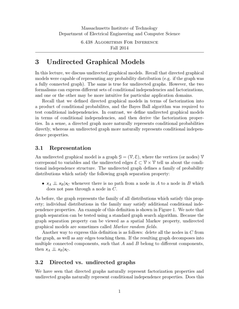
pendence properties. An example of this definition is shown in Figure 1. We note that
graph separation can be tested using a standard graph search algorithm. Because the
graph separation property can be viewed as a spatial Markov property, undirected
graphical models are sometimes called Markov random fields.
Another way to express this definition is as follows: delete all the nodes in C from
the graph, as well as any edges touching them. If the resulting graph decomposes into
multiple connected components, such that A and B belong to different components,
then xA ⊥⊥ xB |xC .
3.2
Directed vs. undirected graphs
We have seen that directed graphs naturally represent factorization properties and
undirected graphs naturally represent conditional independence properties. Does this
1
(a)
A
C
B
(b)
A
B
Figure 1: (a) This undirected graphical model expresses the conditional independence
property xA ⊥⊥ xB |xC . (b) When the shaded nodes are removed, the graph decomposes
into multiple connected components, such that A and B belong to disjoint sets of
components.
mean that we should always use directed graphs when we have conditional probability
distributions and undirected graphs when we have conditional independencies? No
—it turns out that each formalism can represent certain families of distributions that
the other cannot.
For example, consider the following graph.
w
y
x
z
Let’s try to construct a directed graph to represent the same family of distributions
(i.e. the same set of conditional independencies). First, note that it must contain
at least the same set of edges as the undirected graph, because any pair of variables
connected by an edge depend on each other regardless of whether or not any of the
other variables are observed. In order for the graph to be acyclic, one of the nodes
must come last in a topological ordering; without loss of generality, let’s suppose it is
node z. Then z has two incoming edges. Now, no matter what directions we assign to
the remaining two edges, we cannot guarantee the property x ⊥⊥ y |w , z (which holds
in the undirected graph), because the Bayes Ball can pass along the path x → z ← y
when z is observed. Therefore, there is no directed graph that expresses the same set
of conditional independencies as the undirected one.
What about the reverse case — can every directed graph be translated into an
undirected one while preserving conditional independencies? No, as the example of
the v-structure shows:
2
Figure 2: Part of an undirected graphical model for an image processing task, image
superresolution. Nodes correspond to pixels, and every fourth pixel is observed.
x
z
y
We saw in Lecture 2 that x ⊥⊥ z, but not x ⊥⊥ z|y . By contrast, undirected graphical
models have a certain monotonicity property: when additional nodes are observed,
the new set of conditional independencies is a strict superset of the old one. Therefore,
no undirected graph can represent the same family of distributions as a v-structure.
An example of a domain more naturally represented using undirected rather than
directed graphs is image processing. For instance, consider the problem of image
superresolution, where we wish to double the number of pixels along each dimension.
We formulate the graphical model shown in Figure 2, where the nodes correspond
to pixels, and undirected edges connect each pair of neighboring pixels. This graph
represents the assumption that each pixel is independent of the rest of the image
given its four neighboring pixels. In the superresolution task, we may treat every
fourth pixel as observed, as shown in the Figure 2.
3.3
Parameterization
Like directed graphical models, undirected graphical models can be characterized
either in terms of conditional independence properties or in terms of factorization.
Unlike directed graphical models, undirected graphical models do not have a natu­
ral factorization into a product of conditional probabilities. Instead, we represent
the distribution as a product of funcations called potentials, times a normalization
constant.
To motivate this factorization, consider a graph with no edge between nodes xi
3
and xj . By definition, xi ⊥⊥ xj |xrest , where xrest is shorhand for all the other nodes in
the graph. We find that
pxall = pxi ,xj |xrest pxrest
= px1 |xrest px2 |xrest pxrest .
Therefore, we conclude that the joint distribution can be factorized in such a way
that xi and xj are in different factors.
This motivates the following factorization criterion. A clique is a fully connected
set of nodes. A maximal clique is a clique that is not a strict subset of another clique.
Given a set of variables x1 , . . . , xN and a set C of maximal cliques, define the following
representation of the joint distribution:
px (x) ∝
ψxC (xC ),
C∈C
=
1
Z
ψxC (xC ).
(1)
C∈C
In this representation, Z is called the partition function, and is chosen such that the
probabilities corresponding to all joint assignments sum to 1. The functions ψ can be
any nonnegative valued functions (i.e. do not need to sum to 1), and are sometimes
referred to as compatibilities.
The partition function Z can be written explicitly as
Z=
ψxC (xC ).
x
C∈C
This sum can be quite expensive to evaluate. Fortunately, for many calculations, such
as conditional probabilities and finding the most likely joint assignment, we do not
need it. For other calculations, such as learning the parameters ψ, we do need it.
The complexity of description (number of parameters) is given by:
|X||C| ≈ |X|max |C| .
As with directed graphical models, the main determinant of the complexity is the
number of variables involved in each term of the factorization.1
So far, we have defined an arbitrary factorization property based on the graph
structure. Is this related to our earlier definition of undirected graphical models in
terms of conditional independencies? The relationship was formally established by
the following theorem.
1
Strictly speaking, this approximation does not always hold, as the number of maximal cliques
may be exponential in the number of variables. An example of this is given in one of the homeworks.
However, it is a good rule of thumb for graphs that arise in practice.
4
Theorem 1 (Hammersley-Clifford) A strictly positive distribution p (i.e. px (x) >
0 for all joint assignments x) satisfies the graph separation property from our defini­
tion of undirected graphical models if and only if it can be represented in the factorized
form (1).
Proof:
One direction, the factorization (1) implying satisfaction of the graph separation criterion,
is straightforward. The other direction requires non-trivial arguments. For it, we shall
provide proof for binary Markov random field, i.e. x ∈ {0, 1}N . This proof is adapted from
[Grimmet, A Theorem about Random Fields, BULL. LONDON MATH. SOC, 5 (1973),
81-84].
Now any x ∈ {0, 1}N is equivalent to a set S(x) ≡ S ⊆ V = {1, . . . , N }, where S(x) = {i ∈
V : xi = 1}. With this in mind, the probability distribution of X over {0, 1}N is equivalent
to probability distribution over the set of all subsets of V , 2V . To that end, let us start by
defining
X
Q(S) =
(−1)|S−A| log p XA = 1, XV \A = 0)
(2)
A⊆S
where 1 and 0 are vectors of all ones and zeros respectively (of appropriate length). Ac­
cordingly,
Q(∅) = log p(X = 0).
We claim that if S ⊂ V is not a clique of the graphical model G, then
Q(S) = 0.
(3)
To prove this, we shall use the fact that X is a Markov Random Field with respect to G.
Now, since S is not a clique, there exists i, j ∈ S so that (i, j) ∈
/ E. Now consider
X
Q(S) =
(−1)|S−A| log p XA = 1, XV \A = 0)
A⊆S
=
X
B⊂S:i,j ∈B
/
(−1)|S−B| log
p XB = 1, XV \B = 0) × p XB∪{i,j} = 1, XV \B∪{i,j} = 0)
p XB∪{i} = 1, XV \B∪{i} = 0) × p XB∪{j} = 1, XV \B∪{j} = 0)
(4)
With notation ai,j = p XB∪{i,j} = 1, XV \B∪{i,j } = 0), ai = p XB∪{i} = 1, XV \B∪{i} = 0),
aj = p XB∪{j} = 1, XV \B∪{j} = 0), and a0 = p XB = 1, XV \B = 0), we have
p Xi = 1, Xj = 1, XB = 1, XV \B∪{i,j} = 0)
ai,j
=
aj + ai,j
p Xj = 1, XB = 1, XV \B∪{i,j} = 0)
= p Xi = 1|Xj = 1, XB = 1, XV \B∪{i,j} = 0)
= p Xi = 1|XB = 1, XV \B∪{i,j} = 0),
5
(5)
.
where in the last equality, we have used the fact that (i, j) ∈
/ E and hence Xi is independent
of Xj condition on the assignment of all other variables fixed. In a very similar manner,
ai
= p Xi = 1|XB = 1, XV \B∪{i,j} = 0).
a0 + ai
From (5)-(6), we conclude that
(6)
aj
a0
=
ai,j
ai
therefore in (4) we have that Q(S) = 0. This establishes the claim that Q(S) = 0 if S ⊂ V
is not a clique. From (2) and with notation G(A) = log p XA = 1, XV \A = 0) for all A ⊂ V
and µ(S, A) = (−1)| S − A| any S, A ⊂ V such that A ⊂ S, we can re-write (2) as
X
Q(S) =
µ(S, A)G(A).
(7)
A⊂S
Therefore,
X
Q(A) =
A⊂S
X X
µ(A, B)G(B)
A⊂S B⊂A
=
X
X
µ(A, B)G(B)
B⊂S B⊂A⊂S
=
X
B⊂S
=
X
X
G(B)
µ(A, B)
s
B⊂A⊂S
G(B)δ(B, S)
B⊂S
= G(S),
(8)
where δ(B, S) is 1 if B = S and 0 otherwise. To see the second last equality, note that given
6 S, all A such that B ⊂ A ⊂ S can be decomposed amongst
B ⊂ S and B =
s sets so that
|A − B| = £, for 0 ≤ £ ≤ k ≡ |S − B|. The number A with |A − B| = £, is k£ . Therefore,
X
µ(A, B) =
B⊂A⊂S
k
X
(−1)£
£=0
k
£
= 1 − 1)k = 0.
(9)
Of course, when B = S, the above is equal to 1 trivially. Thus, we have that for any
x ∈ {0, 1}N ,
log p X = x) = G(N (x))
X
=
Q(S),
S⊂N (x):S clique
(10)
where N (x) = {i ∈ V : xi = 1}. In summary,
X
p X = x) ∝ exp
S⊂V :S
6
clique
s
PS (x) ,
(11)
x1
...
x3
x2
xN
1
xN
Figure 3: A one dimensional Ising model.
where the potential function PS : {0, 1}|S| → R, for each clique S ⊂ V is defined as
Q(S)
0
PS (x) =
if S ⊂ N (x)
otherwise.
(12)
This completes the proof.
3.4
Energy interpretation
We now note some connections to statistical physics. The factorization (1) can be
rewritten as
pX (x) =
1
exp − H(x) .
Z
X
1
exp −
HC (xC ) ,
Z
C∈C
a form known as the Boltzmann distribution. H(x) is sometimes called the Hamil­
tonian, and relates to the energy of the state x. Effectively, global configurations
with low energy are favored over those with high energy. One well-studied example
is the Ising model, for which the one-dimensional case is shown in Figure 3. In the
one-dimensional case, the variables x1 , . . . , xN , called spins, are arranged in a chain,
and take on values in {+, −}. The pairwise compatibilities either favor or punish
states where neighboring spins are identical. For instance, we may define
Hxi ,xi+1 =
3/2 1/5
1/5 3/2
.
There exist factorizations of distributions that cannot be represented by either
directed or undirected graphical models. In order to model some such distributions,
we will introduce the factor graph in the next lecture. (Note that this does not imply
that there exist distributions which cannot be represented in either formalism. In
fact, in both formalisms, fully connected graphs can represent any distribution. This
observation is uninteresting, because the very point of graphical models is to com­
pactly represent distributions in ways that support efficient learning and inference.)
The existence of three separate formalisms for representing families of distributions
as graphs is a sign of the immaturity of the field.
7
MIT OpenCourseWare
http://ocw.mit.edu
6.438 Algorithms for Inference
Fall 2014
For information about citing these materials or our Terms of Use, visit: http://ocw.mit.edu/terms.