Massachusetts Institute of Technology
Department of Electrical Engineering and Computer Science
6.245: MULTIVARIABLE CONTROL SYSTEMS
by A. Megretski
Problem Set 2 Solutions
1
Problem 2.1
For each of the statements below decide whether it is true or false.
For a true statement, sketch a proof. For a false statement, give a
counterexample.
(a) H2 norm of a stable finite order CT LTI state space model is never
larger than 100 times its H-Infinity norm.
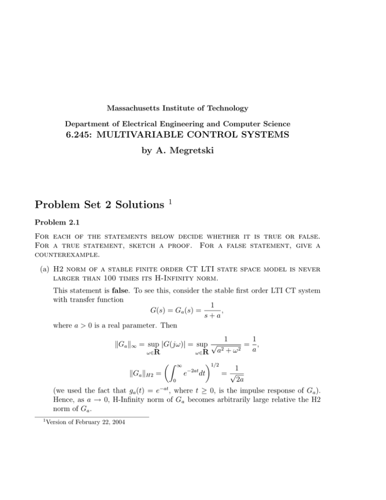
This statement is false. To see this, consider the stable first order LTI CT system
with transfer function
1
G(s) = Ga (s) =
,
s + a
where a > 0 is a real parameter. Then
1
1
∈Ga ∈� = sup |G(j�)| = sup �
= ,
2
2
a
a +�
��R
��R
�
�
�1/2
1
−2at
∈Ga ∈H2 =
e
dt
=�
2a
0
(we used the fact that ga (t) = e−at , where t √ 0, is the impulse response of Ga ).
Hence, as a � 0, H-Infinity norm of Ga becomes arbitrarily large relative the H2
norm of Ga .
1
Version of February 22, 2004
2
(b) H-Infinity norm of a stable finite order CT LTI state space model is
never larger than 100 times its H2 norm.
This statement is false. To see this, use Ga from (a) with a � →.
(c) H2 norm of a stable finite order DT LTI state space model is never
larger than 100 times its H-Infinity norm.
The statement is true for SISO models, because
�
�
1
1
j� 2
2
|G(e )| d� ∀
max{|G(ej� )|2 }d� = ∈G∈2� .
∈G∈H2 =
2� −�
2� −� �
However, for MIMO systems, the statement is false. To see this, consider G = G(z)
which is�an n-by-n identity matrix: its H-Infinity norm equals 1 while the H2 norm
equals n.
(d) H-Infinity norm of a stable finite order DT LTI state space model is
never larger than 100 times its H2 norm.
This statement is false. To see this, consider the stable first order LTI DT system
with transfer function
1
H(z) = Ha (z) =
,
1 − a/z
where a ≤ (0, 1) is a real parameter. Then
1
∈Ha ∈� = sup |H(ej� )| =
,
1−a
��R
∈Ha ∈H2 =
�
�
�
a2k
k=0
�1/2
=�
1
1 − a2
(we used the fact that ha [k] = ak , where k √ 0, is the impulse response of Ha ).
Hence, as a � 1, H-Infinity norm of Ha becomes arbitrarily large relative the H2
norm of Ha .
Problem 2.2
For continuous time (non-LTI) systems Sa with scalar input f = f (t) and
scalar output g = g(t), described below, find their L2 gains, as functions
of parameter a > 0. Support your answer with arguments (typically,
3
to show that L2 gain of a system equals, say, 0.5, one has to find input/output pairs of infinite energy (i.e. not converging to zero) for
which the asymptotic (as time converges to infinity) output-to-input en­
ergy ratio is arbitrarily close to 0.25 = 0.52 , and, in addition, to show
that the asymptotic energy ratio cannot be larger than 0.5).
(a) g(t) = a sin(f (t));
L2 gain equals a.
To see that the L2 gain cannot be larger, note that
| sin(y)| ∀ |y |
for all real y. Hence
T
2
|g(t)| dt =
0
T
2
0
|a sin(f (t))| dt ∀ a
2
T
0
|f (t)|2 dt.
To see that the L2 gain cannot be smaller, consider input f (t) ≥ e, where π > 0 is
a small parameter. Then, for every � we have
T
{� 2 |f (t)|2 − |g(t)|2 }dt = T (� 2 π2 − a2 sin2 (π)),
0
which will converge to minus infinity as T � → unless
� 2 π2 − a2 sin2 (π) √ 0.
Since this inequality must be satisfied for all π whenever � is larger than the L2
gain, we have � 2 √ a2 .
(b) g(t) = f (at) sin(t);
�
For a ∀ 1 L2 gain equals 1/ a. For a > 1 the gain is infinite (and the system is
not causal).
�
To see that L2 gain does not exceed 1/ a for a ∀ 1, note that
T
T
2
|g(t)| dt =
|f (at)|2 sin2 (t)dt
0
∀
T
0
1
|f (at)| dt =
a
2
0
aT
1
|f (t)| dt ∀
a
2
0
T
0
|f (t)|2 dt.
4
�
To see that L2 gain is not smaller than 1/ a for a ∀ 1, consider
� −1/2
k
, t ≤ [(k + 21 )� − π, (k + 12 )� + π], k ≤ {1, 2, . . . },
f (t) =
0,
otherwise.
(The main idea is that f (t) should be zero when | sin(t)| is not close to 1, and the
energy of f (t) on the interval [aT, T ] should converge to zero as T � →, while the
total energy of f should be infinite.) Then
T
T
T
2
2
2
2
2
{� |f (t)| − |g(t)| }dt ∀
� |f (t)| dt −
cos2 (π)|f (at)|2 dt
0
0
0
aT
T
cos2 (π)
|f (t)|2 dt + � 2
|f (t)|2 dt,
a
0
aT
which converges to −→ as T � → unless � 2 √ cos2 (π)/a. Since π > 0 can be
arbitrarily small, g √ 1/a for a √ 1.
=
�
�
�2 −
To show that L2 gain is infinite for a > 1, consider
� k
r , t ≤ [(k + 21 )� − π, (k + 12 )� + π], k ≤ {1, 2, . . . },
f (t) =
0, otherwise,
where r ∞ 1 is a parameter. It is easy to see that, when r � → is sufficiently large
compared to �, the integrals
T
{� 2 |f (t)|2 − |g(t)|
2 }dt
0
converge to minus infinity as T � →.
(c) g(t) = af (t) − |f (t − 1)|.
L2 gain equals 1 + a.
To see that L2 gain does not exceed 1 + a, note that
�
�
|ax + y |2 ∀ (1 + a) a|x|2 + |y |2 � x, y,
and hence
T
2
0
|g(t)| dt ∀ (1 + a)a
∀ (1 + a)2
T
2
0
|f (t)| dt + (1 + a)
T
0
|f (t)|2 dt +
0
−1
T
0
|f (t − 1)|2 dt
|f (t)|2 dt.
To see that L2 gain is not smaller than 1 + a, consider the case when f (t) ≥ −1,
and hence g(t) ≥ −(1 + a).
5
Problem 2.3
Continuous time signal q = q(t) is the output of a pure double integrator
system with input f1 = f1 (t), and g(t) = q(t) + bf2 (t), where b > 0 is a known
constant (do the calculations for b = 0.1 and b = 10). Find an LTI filter
F = F (s) which takes g = g(t) as an input and outputs an estimate q̂ = q̂(t)
of q = q(t), which is “good” in one of the following interpretations:
(a) Assuming that f = [f1 ; f2 ] is white noise, minimize the asymptotic value
of the variance of the estimation error e = q − q̂.
(b) Minimize the L2 gain from f = [f1 ; f2 ] to the estimation error e = q − q̂
with accuracy 10 percent.
For a system with state space equations
ẋ(t) = A0 x(t) + B10 w(t)
and sensor output
0
w(t),
y0 (t) = C20 x(t) + D21
a standard observer has the format
x(t)
ˆ˙
= A0 x(t)
ˆ + L(C20 x(t)
ˆ − y0 (t)),
where matrix L is chosen in such way that A0 + LC20 is a Hurwitz matrix. Note that here
x̂ is a result of applying an LTI transformation to y. Hence
d(t) = y0 (t) − C20 x(t)
ˆ
is a result of applying an LTI transformation to y0 (t), and, reciprocally, y0 (t) is a result of
applying an LTI transformation to d(t). Therefore, designing an LTI filter F with input
y0 output v = F y0 , to be an optimal estimate of a state component q(t) = C10 x(t) can be
reduced to designing an LTI filter Fd with input d(t) and output vd = Fd d, to be a good
estimate of qd (t) = q(t) − C10 x(t):
ˆ
the relation between vd and v will be
ˆ + vd (t).
v(t) = C10 x(t)
The relation between w, d, and qd is given by
0
0
ė = (A0 + LC20 )e + (B10 + LD21
)w, d = C20 e + D21
w, qd = C10 e,
6
where e(t) = x(t) − x̂(t) plays the role of system state. The task of finding an optimal or
suboptimal estimator for qd based on measuring d can be formulated as a standard LTI
feedback optimization setup with
0
0
A = A0 +LC20 , B1 = B10 +LD21
, B2 = 0, C1 = C10 , D11 = 0, D12 = I, C2 = C20 , D21 = D21
, D22 = 0.
To implement the filter optimization approach using MATLAB, we use a design
SIMULINK model ps2 3a.mdl,
1
1/s^2
(s+1)/(s^2+s+1)
w1
plant
2
w2
2
3
1
y
u
e
observer
b
Gain
handled by M-function ps2 3.mdl:
function [Fh2,Fhi,Eh2,Ehi]=ps2_3(b)
% function ps2_3(b)
%
% solution for Problem 2.3 in 6.245/Spring 2004
if nargin<1, b=1; end
assignin(’base’,’b’,b);
s=tf(’s’);
assignin(’base’,’s’,s);
load_system(’ps2_3a’);
[a,b,c,d]=linmod(’ps2_3a’);
close_system(’ps2_3a’);
[ar,br,cr,dr]=ssdata(minreal(ss(a,b,c,d)));
p=pck(ar,br,cr,dr);
nmeas=1;
ncon=1;
7
ricmethd=2;
quiet=0;
[kh2,gh2]=h2syn(p,nmeas,ncon,ricmethd,quiet);
[ah2,bh2,ch2,dh2]=unpck(kh2);
[ag,bg,cg,dg]=unpck(gh2);
Kh2=ss(ah2,bh2,ch2,dh2);
G=(s+1)/(s^2+s+1);
disp(’H2 controller:’)
Fh2=tf(minreal(Kh2*(G-1)+G))
Eh2=tf(minreal(ss(ag,bg,cg,dg)));
gmin=0;
gmax=norm(Eh2,Inf);
tol=0.01;
epr=1e-10;
epp=1e-6;
[khinf,ghinf]=hinfsyn(p,nmeas,ncon,gmin,gmax,tol,ricmethd,epr,epp,quiet);
[ahi,bhi,chi,dhi]=unpck(khinf);
[ag,bg,cg,dg]=unpck(ghinf);
Ehi=tf(minreal(ss(ag,bg,cg,dg)));
Khi=ss(ahi,bhi,chi,dhi);
disp(’H-Infinity controller:’)
Fhi=tf(minreal(Khi*(G-1)+G))
Note the need for using minreal.m: MATLAB does not eliminate uncontrollable/unobservable
states automatically.