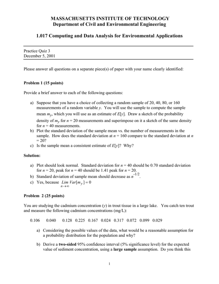
MASSACHUSETTS INSTITUTE OF TECHNOLOGY
Department of Civil and Environmental Engineering
1.017 Computing and Data Analysis for Environmental Applications
Practice Quiz 3
December 5, 2001
Please answer all questions on a separate piece(s) of paper with your name clearly identified:
Problem 1 (15 points)
Provide a brief answer to each of the following questions:
a) Suppose that you have a choice of collecting a random sample of 20, 40, 80, or 160
measurements of a random variable y. You will use the sample to compute the sample
mean my, which you will use as an estimate of E[y]. Draw a sketch of the probability
density of my for n = 20 measurements and superimpose on it a sketch of the same density
for n = 40 measurements.
b) Plot the standard deviation of the sample mean vs. the number of measurements in the
sample. How does the standard deviation at n = 160 compare to the standard deviation at n
= 20?
c) Is the sample mean a consistent estimate of E[y]? Why?
Solution:
a) Plot should look normal. Standard deviation for n = 40 should be 0.70 standard deviation
for n = 20, peak for n = 40 should be 1.41 peak for n = 20.
-1/2
b) Standard deviation of sample mean should decrease as n .
c) Yes, because Lim Var[m y ] = 0
n→∞
Problem 2 (25 points)
You are studying the cadmium concentration (y) in trout tissue in a large lake. You catch ten trout
and measure the following cadmium concentrations (mg/L):
0.106
0.040
0.128 0.225 0.167 0.024 0.317 0.072 0.099 0.029
a) Considering the possible values of the data, what would be a reasonable assumption for
a probability distribution for the population and why?
b) Derive a two-sided 95% confidence interval (5% significance level) for the expected
value of sediment concentration, using a large sample assumption. Do you think this
1
assumption is justified? Why? Note that the 2.5% lower and upper critical values for a
unit normal probability distribution are –1.96 and +1.96.
c) Carry out a two-sided large sample test of the hypothesis H0: E[y] = 0.2. Is H0
accepted or rejected at a 5% significance level?
Solution:
a) A histogram of the data suggest that y is exponentially distributed.
b) Sample mean is my = 0.12
Sample standard deviation is sy = 0.094
If we adopt a large sample approximation we assume that the sample mean is normally
distributed with mean E[my] = E[y] ((the unknown true mean) and standard deviation
SD[my] = sy/n1/2 = 0.094/(10)1/2 = 0.03. The critical points for a two-sided 95% confidence
interval are given by:
myl,0.95 = my - SD[my](1.96) = 0.12 - (0.03)(1.96) = 0.063
myu,0.95 = my + SD[my](1.96) = 0.12 + (0.03)(1.96) = 0.18
So we infer from the data that E[y] probably lies in the interval between 0.063 and 0.18.
Based on our experience with stochastic simulation of small exponential samples, the large
sample approximation is reasonably good for samples as small as n = 10 at significance
levels of 0.05 or larger.
c) Find the two-sided large sample acceptance region for a significance level of 5% from:
myl,0.95 = E[y|H0] - SD[my](1.96) = 0.2 - (0.03)(1.96) = 0.14
myu,0.95 = E[y|H0] + SD[my](1.96) = 0.2 + (0.03)(1.96) = 0.26
Since the sample mean estimate my = 0.12 lies outside the acceptance region we reject H0.
Problem 3 (30 points)
Consider the following 4 values of the independent variable (time) and the dependent variable
(change in total dry biomass relative to long-term average) in a temperate forest:
Time (months):
2.0
2.5
4.0
8.0
Biomass (Kg/m2):
2.7
3.3 -1.6
9.0
Compare the following two regression models by following the indicated steps:
y L ( x, a 2 ) = a 2 x
2
y S ( x, a 2 ) = a 2 Sin( x)
a) For each model, derive the least-squares estimate for a2. You can do this by minimizing the
sum-of-squares error directly or by using the following expression:
H ′Hâ2 = H ′y
where:
H = [ x1,…, x4 ] = [2.0
2.5
4.0
H = [ sin(x1),…, sin(x4)] = [ 0.91
8.0 ]
0.60
for the first model
-0.76 0.99 ] for the second model
b) Plot the regression line over the range of measurement x values and calculate the sum-ofsquared errors or SSE (the easiest way to do this is to read the error values directly off your
plot). Which line gives a smaller SSE?
c) Which regression model do you prefer? Why?
Solution:
% Quiz 3, Solution to Problem 4
function quiz01_3sol4
% generate data
xmeas=[2,2.5,4,8]
ymeas=xmeas.*sin(xmeas)+2*normrnd(0,1,1,4)
hL=xmeas'
hS=sin(xmeas)'
a2Lhat=inv(hL'*hL)*(hL'*ymeas')
a2Lhat=(hL'*hL)\(hL'*ymeas')
a2Shat=(hS'*hS)\(hS'*ymeas')
SSEL=(ymeas-a2Lhat*xmeas)*(ymeas-a2Lhat*xmeas)'
SSES=(ymeas-a2Shat*sin(xmeas))*(ymeas-a2Shat*sin(xmeas))'
x=[1:.01:9];
yL=a2Lhat*x;
yS=a2Shat*sin(x);
close all
figure
plot(xmeas,ymeas,'*')
hold on
plot(x,yL,'r')
hold on
plot(x,yS,'b')
return
3
a2Lhat =
0.8781
a2Shat =
5.3151
SSEL =
32.1493
SSES =
24.4308
Problem 4 (30 points)
Consider the following random sample of 6 measurements of a random variable y distributed
uniformly between 0 and c:
0.8775
0.0319
0.8537
0.7946
0.3409
0.0080
a) Use this sample to derive an appropriate estimate of c, the upper bound of the random
variable y.
b) Write a stochastic simulation program that evaluates and plots on a normal probability scale
the cumulative distribution function of the estimator you used to compute c.
c) Suppose that your program produces the following plot when a value of c = 1.5 is used in
the uniform random number generator used to generate the replicates. Indicate on the plot
(with lines and arrows) how you would derive the p value for a two sided test of the
hypothesis H0: c = 1.5 when your estimate of c is obtained from the above sample. What is
the p value? Would you reject the hypothesis? Why?
d) Do you think a large sample approximation is valid for this hypothesis testing problem?
Why?
4
Solution
zeta =
0.9689
% Quiz 3, Solution to Problem 5
function quiz01_3sol5
% specify sample data and compute sample estimate
samp=[ 0.8775
0.0319
0.8537
0.7946
0.3409
zeta=2*mean(samp)
n=6
nrep=10000
close all
c=1.5
% replicate loop
for i=1:nrep
ymc=unifrnd(0,c,1,n);
cmc(i)=2*mean(ymc);
end
% construct CDF for hypothesized c
normplot(cmc)
return
5
0.0080]
ξ = 0.97
p/2 = 0.05
p = 0.1
6