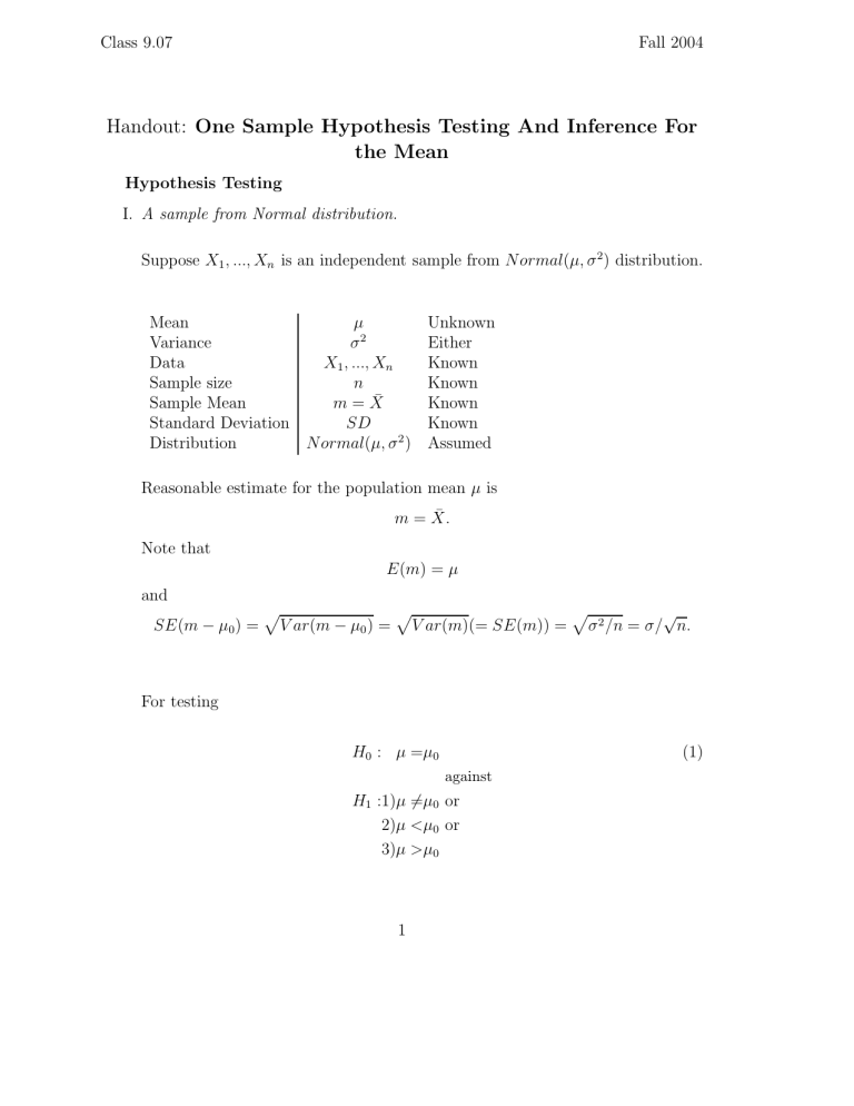
Class 9.07
Fall 2004
Handout: One Sample Hypothesis Testing And Inference For
the Mean
Hypothesis Testing
I. A sample from Normal distribution.
Suppose X1 , ..., Xn is an independent sample from Normal(µ, σ 2 ) distribution.
Mean
µ
Variance
σ2
Data
X1 , ..., Xn
Sample size
n
¯
Sample Mean
m=X
Standard Deviation
SD
Distribution
Normal(µ, σ 2 )
Unknown
Either
Known
Known
Known
Known
Assumed
Reasonable estimate for the population mean µ is
¯
m = X.
Note that
E(m) = µ
and
SE(m − µ0 ) =
�
V ar(m − µ0 ) =
�
�
√
V ar(m)(= SE(m)) = σ 2 /n = σ/ n.
For testing
H0 : µ =µ0
(1)
against
H1 :1)µ =µ0 or
2)µ <µ0 or
3)µ >µ0
1
use
test statistics dobt =
m − µ0
SE(m)
which follows some distribution d∗ .
Theorem. Under the above assumptions about the sample X1 , ..., Xn , for test­
ing test H0 : µ − µ0 = 0 at α - significance level
vs
1) H1 : µ − µ0 =
0. Reject H0 if |d∗obt | ≥ d∗crit (α/2)
2) H1 : µ − µ0 < 0. Reject H0 if d∗obt ≤ −d∗crit (α)
3) H1 : µ − µ0 > 0. Reject H0 if d∗obt ≥ d∗crit(α)
Computation of SE(m) and choice of distribution d∗ :
1. σ is known √
SE(m) = σ/ n
Test statistics d∗obt = zobt =
m−µ
√0
σ/ n
follows standard Normal distribution z.
2. σ is unknown, but n is large (≥ 30)
In this case can
assumption.
√ omit Normality
√
SE(m) = σ/ n ≈ SD/ n and
m−µ
√0 approximately follows standard Normal
test statistics d∗obt = zobt = SD/
n
distribution z.
3. σ is unknown,
√ and n is not
√ large enough (≤ 30)
SE(m) = σ/ n ≈ SD/ n and
m−µ
√0 follows t distribution with df = n − 1
test Statistics d∗obt = tobt = SD/
n
degrees of freedom.
II. Proportions
For a random variable X drawn from a Binomial(n, p) distribution, let p̄ =
X/n. For testing
2
H0 : p =p0
(2)
against
H1 :1)p =p0 or
2)p <p0 or
3)p >p0
use test statistics dobt =
p̄−p0
.
SE(¯
p−p0 )
Since for a Binomial(n, p) random variable X and p̄ = X/n, V ar(¯
p − p0 ) =
p(1−p)
V ar(¯
p) = n , for H0 true (that is, p = p0 ) have
SE(¯
p − p0 ) =
Then
�
�
p − p0 ) =
V ar(¯
p0 (1 − p0 )
n
p̄ − p0
test statistics d∗obt = zobt = �
p0 (1−p0 )
n
has approximately Normal z distribution if np, n(1 − p) ≥ 10.
3
Confidence Intervals
For a test statistics d∗obt =
m−µ0
SE(m)
we reject H0 if |d∗obt | ≥ d∗crit (α/2). If
∗
< d∗crit (α/2)
−d∗crit (α/2) < dobt
we conclude that evidence against H0 is not statistically significant at α - significance
level.
Conficence interval for µ is computed by inverting non-rejection region
m − µ0
∗
< dcrit
(α/2)
SE(m)
−d∗crit (α/2)SE(m) < m − µ0 < d∗crit(α/2)SE(m)
−d∗crit (α/2) <
with (1 − α)100% confidence interval for µ:
(m − d∗crit (α/2)SE(m); m + d∗crit (α/2)SE(m))
4