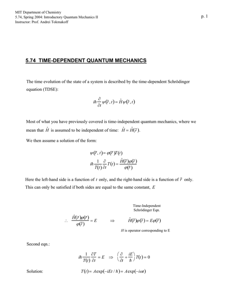
MIT Department of Chemistry
5.74, Spring 2004: Introductory Quantum Mechanics II
Instructor: Prof. Andrei Tokmakoff
p. 1
5.74 TIME-DEPENDENT QUANTUM MECHANICS
The time evolution of the state of a system is described by the time-dependent Schrödinger
equation (TDSE):
∂
ψ (r , t ) = Ĥψ (r , t )
∂t
i
Most of what you have previously covered is time-independent quantum mechanics, where we
mean that Ĥ is assumed to be independent of time: Ĥ = Hˆ (r ).
We then assume a solution of the form:
ψ (r , t ) = ϕ (r )T (t )
i
1 ∂
Hˆ (r )ϕ (r )
T (t ) =
ϕ (r )
T(t ) ∂t
Here the left-hand side is a function of t only, and the right-hand side is a function of r only.
This can only be satisfied if both sides are equal to the same constant, E
Time-Independent
Schrödinger Eqn.
∴
Hˆ (r )ϕ (r )
=E
ϕ (r )
⇒
Hˆ (r )ϕ (r ) = Eϕ (r )
H is operator corresponding to E
Second eqn.:
i
Solution:
1 ∂T
 ∂ iE 
T(t ) = 0
=E ⇒
+


∂t
T(t ) ∂t
T (t ) = Aexp (−iEt / ) = Aexp (−iωt )
p. 2
So, for a set of eigenvectors ϕ n (r ) with corresponding eigenvalues En , there are a set of
corresponding eigensolutions to the TDSE.
ψ n (r , t ) = anϕ n (r ) exp(− iω nt )
ωn = En /
The probability density
P = ∫ ψ (r, t )ψ (r , t )dr = ψ (r , t )ψ (r , t )
*
may be time dependent for ψ ( r , t ) , but is independent of time for the eigenfunctions ψ n ( r , t ) .
Therefore, ϕ (r ) are called stationary states.
However, more generally a system may be represented as a linear combination of eigenstates:
ψ (r , t ) = ∑ cnψ n (r , t ) = ∑ cn e− iω tϕ n (r )
n
n
n
For such a case, the probability density will oscillate with time: coherence.
e.g., two eigenstates
ψ (r, t ) = c1ϕ 1e −iω t + c2 ϕ 2 e− iω
1
2
t
p(t ) = ψ *ψ = c1ϕ1 + c2ϕ 2 + c1* c2ϕ 1*ϕ 2 e− i(ω2 −ω1 t ) + c2 *c1ϕ2 *ϕ 1e +i (ω 2 −ω 1 )t
2
2
probability density oscillates as cos(ω 2 − ω1 )t
This is a simple example of coherence (coherent superposition state). Including momentum (a
wavevector) of particle leads to a wavepacket.
p. 3
TIME EVOLUTION OPERATOR
More generally, we want to understand how the wavefunction evolves with time. The TDSE is
linear in time. Since the TDSE is deterministic, we will define an operator that describes the
dynamics of the system:
ψ (t ) = U (t,t 0 )ψ (t0 )
For the time-independent Hamiltonian:
∂
iH
ψ (r , t ) + ψ (r , t ) = 0
∂t
(1)
To solve this, we will define an operator T = exp(−iHt / ), which is a function of an operator.
A function of an operator is defined through its expansion in a Taylor series:
T = exp[−iHt
]=
1−
iHt
1  iHt  2
+
−

2! 
= f (H)
Multiplying eq. 1 from the left by T −1 = exp (iHt / ) we have:
∂
∂t

  iHt 
ψ (r , t ) = 0
exp 



integrating t 0 → t :
exp 

iHt 
iHt
ψ r , t − exp 0  ψ (r , t 0 ) = 0
 ( )


 −H(t − t0 )
 ψ (r, t 0 ) = U (t, t0 )ψ (r, t0 )

ψ (r, t ) = exp 
For functions of an operator A :
Given a set of eigenvalues and eigenvectors of A , i.e.,
()
Aϕ n = anϕ n , you can show by expanding the function as a polynomial that f  ϕ n = f (an )ϕ n
p. 4
∴ ψ n (r , t ) = e
− En (t − t0 )/
ψ n (r, t0 )
or, alternatively, if we substitute the projection operator (identity relationship)
U ( t, t 0 ) = e
−iH ( t −t 0 ) /
∑ϕ
n
ϕn
ωn =
n
= ∑e
− iωn ( t − t 0 )
ϕn ϕn
En
n
This form is useful when ϕ n are characterized; we’ll develop U(t , t0 ) more later. So now we
can write our time-developing wave-function as
ψ n ( r , t ) = ϕn
∑e
− iωn ( t − t 0 )
∑e
− iωn ( t − t 0 )
ϕn ψ n ( r , t 0 )
n
= ϕn
cn ( t 0 )
n
Time-evolution of a coupled two-level system (2LS)
It is common to reduce or map problem onto a 2LS. We then discard remaining degrees of
freedom, or incorporate them as a heat bath, H = H 0 + H bath .
Let’s discuss the time-evolution of a 2LS with a time-independent Hamiltonian. Consider a 2LS with two (unperturbed) eigenstates ϕ a and ϕ b with eigenenergies ε a and ε b ,
which are then coupled through an interaction Vab .
V
ϕa εa
H = a ε a a + b ε b b + a Vab b + b Vba a
ε
= a
Vba
Vab 

εb 
Since the Hamiltonian is Hermetian, (Hij = H *ji ), we suggest
ε+
2∆
ϕ b εb
ε-
p. 5
Vab = Vba* = Ve − iφ
 ε
H =  a+ iφ
 Ve
Ve − iφ 

εb 
If we define the variables
E=
εa + εb
2
ε − εb
∆= a
2
Then we can solve for the eigenvalues of the coupled systems:
ε ± = E ± ∆2 + V 2
Because the expressions get messy, we don’t choose to find the eigenvectors for the coupled
system, ϕ ± , using this expression. Rather, we use a substitution where we define:
tan 2θ =
V
∆
2θ
∆
(0 < θ < π/2)
1
H = E I + ∆
+ iφ
 tan 2θe
tan 2θe − iφ 

−1

We now find that we can express the eigenvalues as
ε ± = E ± ∆ sec2θ
We now want to find the eigenstates of the Hamiltonian, ϕ ± , H ϕ ± = ε ± ϕ ±
where e.g. ϕ + = c a ϕ a + cb ϕ b :
ϕ+ = cos θ e − iφ / 2 ϕa + sin θ eiφ / 2 ϕb
ϕ− = − sin θ e − iφ / 2 ϕa + cos θ eiφ / 2 ϕb
Orthonormal complete + orthogonal:
ϕa ϕa + ϕ b ϕ b = 1
V
p. 6
Examine the limits:
(a) Weak coupling (V/∆ << 1). Here θ ≈ 0, and ϕ + corresponds to ϕ a perturbed by the Vab
interaction. ϕ− corresponds to ϕb .
( For θ → 0
ϕ + → ϕa ; ϕ − → ϕ b
)
(b) Strong coupling (V/∆ >> 1). Now θ = 45º, and the a/b basis states are indistinguishable.
The eigenstates are symmetric and antisymmetric combinations:
ϕ± ~
1
( ϕ b ± ϕa
2
)
Whether + or − corresponds to the symmetric or asymmetric combination depends on whether V
is positive or negative. (For −V >> ∆, θ = −45°)
We can schematically represent the energies of these states:
ε−Ε
ε+
εa
∆
ε-
These eigenstates exhibit avoided crossing.
εb
p. 7
The time-evolution of this system is given by our time-evolution operator.
U(t , t0 ) = ϕ + e− ω+ (t − t0 ) ϕ + + ϕ − e− iω− (t− t0 ) ϕ −
ω ± = ε±
Now ϕ a and ϕ b are not the eigenstates—preparing ϕ a will lead to time-evolution!
Let’s prepare the system so that it is initially in state ϕ a .
(t0 = 0)
ψ (0) = ϕ a
What is the probability that it is found in state ϕ b at time t ?
Pba (t ) = ϕb ψ (t )
2
= ϕ b U(t, t 0 )ϕ a
2
To evaluate this, you need to know the transformation from the ϕ a,b to the ϕ ± basis, given
above. This gives:
Pba (t ) =
where the Rabi Frequency Ω R =
1
V2
2
2
2 sin Ω Rt
V +∆
∆2 + V 2
Ω R represents the frequency at which probability amplitude oscillates between ϕ a and ϕ b states.
Pba ( t )
V2
V2 + ∆2
0
Notice for V → 0
t = π/ΩR
t
ϕ ± → ϕ a ,b (the stationary states), and there is no time-dependence.
For V >> ∆ , then Ω R =
V
and P = 1 after t =
π
2Ω R
=
π
2V
.
p. 8
TIME-INDEPENDENT HAMILTONIAN
There are two types of values that we often calculate:
Correlation amplitude: C(t ) = β ϕ (t )
measures the resemblance between the state of your system at time t and a target state
2
β . The probability amplitude P(t ) = C(t )
for a set of eigenstates ϕ n
C ( t ) = β ψ ( t ) = β U ( t, t 0 ) ψ ( 0 )
=
∑c
*
m
mj e
−ω j t
j n cn
m,n , j
= ∑ c*m c n e −iωn t
n
Expectation values: A(t ) = ψ (t ) A ψ (t )
ψ (t ) = ∑ e −ω tcn ϕ n =∑ cn ϕ n
n
n
ψ (t ) = ∑ e
n
−ω m t *
m
c ϕm
m
A(t ) = ∑ c*m cn e −iω nmt ϕ m A ϕ n
m, n
= ∑ c*m (t )c n (t )Amn
m, n
E − Em
ω nm = n
ωn − ωm
p. 9
DENSITY MATRIX
For a system described by a wavefunction ψ ( t ) = ∑ c n ( t ) n we showed
n
A(t ) = ψ (t ) A ψ (t )
= ∑ c*m (t )cn (t ) m A n
n, m
We will often find it useful to define a density operator
ρ(t ) ≡ ψ (t ) ψ (t )
= ∑ cn (t )cm* (t ) n m
n,m
= ∑ ρ nm (t ) n m
(by definition)
n,m
ρ n m are the density matrix elements. Substituting, we see that
A(t ) = ∑ Amn ρ nm (t )
n,m
= Tr[A ρ (t )]
Tr (ABC) = Tr(CAB) = Tr(BCA )
Trace Properties: 1) cyclic invariance
2) invariant to unitary transformation
Tr ( S† AS) = Tr ( A )
Pure vs. Mixed States
Why would we need the density matrix? It helps for mixed states.
1) pure states: a system characterized by a wavefunction (previous page)
2) mixed states: not characterized by single wavefunction
> statistical mixtures—ensemble at thermal equilibrium
> independently prepared states
> no phase relationship between elements of mixture p. 10
For an ensemble of systems with a probability pk of occupying quantum state ψ k , with
∑p
k
=1
k
A ( t ) = ∑ pk ψ k ( t ) A ψ k ( t )
k
ρ ( t ) ≡ ∑ pk ψ k ( t ) ψ k ( t )
k
A ( t ) = Tr  Aρ ( t ) 
Properties:
1) ρ is Hermetian ρ *nm = ρ mn
2) Tr (ρ ) = 1 Normalization
3)
Tr (ρ 2 )= 1 for pure state
< 1 for mixed state
Let’s look at the density matrix elements for a mixture:
ρnm = n ρ m = ∑ p k n ψ k
ψk m
k
where ϕk = ∑ c n
k n
n
k
n
c : expansion coefficient for
eigenstate n of wavefunction k
= ∑ p k c kn ( c km )
*
k
= c n c*m
coefficients for eigenstate averaged over mixture
Diagonal elements (n = m)
ρnn = ∑ p k c nk =c n c*n = p n
2
k
probability of finding a system in mixture in state n
POPULATION
(≥ 0 )
p. 11
Off-Diagonal Elements (n ≠ m) —complex—have phase factor
describe the evolution of coherent superpositions.
COHERENCES
For an arbitrary state χ , the expectation value of the density matrix:
χ ρχ
gives the total probability of finding a particle in the pure state χ within the mixture.
We will sometimes refer to the density matrix at thermal equilibrium ρ0 ( or ρeq), which is
characterized by thermally distributed populations in the quantum states
ρnn = p n =
e −βEn
Z
where Z is the partition function. More generally, the density matrix can be defined as
ρ=
where Z = Tr(e−βH). For H n = E n n
e − βH
Z
,
ρnm = n | e −βH | m
= e−βEn δ nn
p. 12
TIME-EVOLUTION OF DENSITY MATRIX
Follows naturally from definition of ρ and T.D.S.E.
∂
−i
ψ = Hψ
∂t
i
∂
ψ = ψ H
∂t
(H
†
= H)
∂ρ ∂
∂
∂

=  ψ ψ  =  ψ  ψ + ψ
ψ
∂t ∂t
∂t
 ∂t

=
−i
Hψ ψ+
i
ψ ψH
∂ρ −i
= [ H, ρ]
∂t
Liouville-Von Neumann Eqn.
For a time-independent Hamiltonian:
ρnm ( t ) = n ρ ( t ) m = n ψ ( t ) ψ ( t ) m
ψ ( t ) = U ( t, t 0 ) ψ ( t 0 ) = ∑ n e
−ωn ( t − t 0 )
n ψ ( t0 )
ni
ρnm ( t ) = e
=e
ωnm =
Populations: ρnn ( t ) = ρnm ( t 0 )
− iωn ( t − t 0 )
− iωnm ( t − t 0 )
n ψ ( t0 ) ψ ( t0 ) m e
ρnm ( t 0 )
En − Em
time-invariant
Coherences: oscillate at energy splitting ωnm
+ iωm ( t − t 0 )