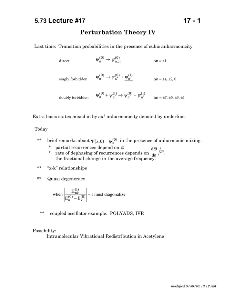
5.73 Lecture #17
17 - 1
Perturbation Theory IV
Last time: Transition probabilities in the presence of cubic anharmonicity
direct
(0)
ψ n(0) → ψ n±1
∆n = ±1
singly forbidden
(1)
ψ n(0) → ψ n(0)
′ + ψ n′
∆n = ±4, ±2, 0
doubly forbidden
(1)
ψ n(0) + ψ n(1)′ → ψ n(0)
′ + ψ n′
∆n = ±7, ±5, ±3, ±1
Extra basis states mixed in by ax3 anharmonicity denoted by underline.
Today
**
brief remarks about Ψ( x, 0) = ψ n(0) in the presence of anharmonic mixing:
* partial recurrences depend on ω
dω
* rate of dephasing of recurrences depends on dn ω ,
the fractional change in the average frequency.
**
“x-k” relationships
**
Quasi degeneracy
when
**
H(1)
nk
(0)
E (0)
n − Ek
≈ 1 must diagonalize
coupled oscillator example: POLYADS, IVR
Possibility:
Intramolecular Vibrational Redistribution in Acetylene
modified 9/30/02 10:12 AM
5.73 Lecture #17
17 - 2
What about Quartic perturbing term bx4?
special
hint
4
Note that E(1)
n = n bx n ≠ 0 and is
directly sensitive to sign of b!
What about wave packet calculations?
ψ n expressed as superposition of ψ k(0) basis state terms
(perturbed eigenstates)
Ψ( x,0) expanded as superposition of ψ k(0) terms
(state prepared at t = 0)
Ψ( x, t ) oscillates at e −iE n t h
(evolving prepared state)
(1)
(2)
E n = E (0)
n + En + En
A state which is initially in a pure ψ n(0) will
dephase, then exhibit partial recurrences at
m2 π
where m is an integer
ω
but recurrence is not perfect since
E n − Em ≠ hω ( n − m)
m2 π ≈ ω n t
not quite
integer
multiples
E n + E n+1
2
decreases as n increases
because
*
*
∴ t recurrence =
time of 1st recurrence will depend on ⟨E⟩!
successive recurrences will occur with larger phase error
for ωn,n–1 vs. ωn+1,n
1st recurrence phase discrepancy is δ
2nd recurrence phase discrepancy is 2δ
etc.
modified 9/30/02 10:12 AM
5.73 Lecture #17
17 - 3
On pages 16-5 through 16-11 I worked out how a block of Heff is corrected so that
“out-of-block” off-diagonal matrix elements can be safely ignored. These
corrections come in two forms:
(i)
Second-order perturbation theory corrections to diagonal matrix
elements. One example is the “x–k” relationships by which the xij
vibrational anharmonicity constants are evaluated in terms of
third and fourth derivatives of V(Q).
(ii)
Van Vleck transformation of “quasi-degenerate” or “resonant”
blocks of Heff. Something analogous to second-order perturbation
theory is used to fold out-of-block off-diagonal matrix elements
into polyad blocks along the diagonal of H. These corrections
occur both on and off the diagonal within these quasi-degenerate
polyad blocks. “Resonance” is not accidental. Once it appears it
affects larger and larger groups of near-degenerate basis states.
Consider the following 3 × 3 example of a Van Vleck transformed Heff:
2
0 5
H =  5 2 0.5


 2 0.5 20 
This H has a 2 ↔2 quasidegenerate block and both
members of this block interact weakly with a nonquasidegenerate remote state.
modified 9/30/02 10:12 AM
5.73 Lecture #17
17 - 4
0 0 0 
H( 0 ) =  0 2 0 


 0 0 20
2
0 5
H(1) =  5 0 0.5


.
2
0
5
0


 22
 −20


1
H( 2 ) =  −
 19

 0

(2)(0.5)
0+2
− 20
2
0.5 2
−18
0





0

 2 2 0.5 2  
 +

 20 18  
0
(1)
nk
(1)
kn ′
( 0)
n′
H H
H = ∑ ( 0)
En + E
( 0)
in-block k
−
E
k
out-of-block
2
( 2)
nn ′
modified 9/30/02 10:12 AM
5.73 Lecture #17
17 - 5
See Ian M. Mills “Vibration-Rotation Structure in Asymmetric- and SymmetricTop Molecules”, pages 115-140 in Molecular Spectroscopy: Modern Research,
Volume I, K. Narahari Rao, and C. Weldon Mathews, Academic, 1972.
Second-order perturbation theory is used to derive the famous “x-k” relationships,
namely the relationship between the second, third, and fourth derivatives of V(Q)
and the normal mode ωi and xij molecular constants.
G(V ) =
∑ ω (v
i
i
+ 1 /2) +
i
1
V (Q) =
2
1
+
24
∑
xij ( vi + 1 /2)( v j + 1 /2)
i,j
i ≥j
∂3V
qr q s qt
∂qr∂q s∂qt
∑
∂2V
∑
∂ 4V
qr q s qt qu
∂qr∂q s∂qt ∂qu
r
rstu
1
2
q
+
r
6
∂qr2
∑
rst
[unrestricted sums: get several identical partial derivatives.] Lengthy derivations:
1 ∂V 1
x ii =
∑
4 −
16 ∂q i 16 s
4
direct firstorder
contribution
from quartic
force constant
 ∂ 3V 
 2 
 ∂q i ∂q s 
2
 (8ω 2i − 3ω 2s ) 

2
2 
 ω s ( 4 ω i − ω s ) 
second-order summation
over cubic force
constants
modified 9/30/02 10:12 AM
5.73 Lecture #17
1 ∂ 4V
1
xij =
−
4 ∂qi2 ∂q 2j 4
17 - 6
∑
t
first-order from quartic
force constant
1
2
∑
t
 ∂ 3V
∂3V
 ∂q 2 ∂q
2
∂
q
i
t

j ∂qt

ωt  −

second-order sum over
∆vi= ∆vj = 0 terms for
cubic force constants
2

3

∂V
2
2
2

ω
ω
ω
ω
−
−
t
t
i
j
 ∂qi ∂q j ∂qt 

(
)

∆ ijt 


second-order sum over all ∆vi = ±1, ∆vj = ±1 terms for cubic force constants
(
)(
)(
)(
∆ ijt = ω i + ω j + ω t ω i − ω j − ω t −ω i + ω j − ω t −ω i − ω j + ω t
)
∆ijt is “Resonance denominator”. When
ωi = ω j + ωt
or
ω j = ωi + ωt
or
ωt = ωi + ω j
perturbation theory blows up. Must go to Heff polyads and diagonalize.
modified 9/30/02 10:12 AM
5.73 Lecture #17
17 - 7
Degenerate and Near Degenerate E (0)
n
*
*
*
Ordinary nondegenerate p.t. treats H as if it can be “diagonalized” by simple
algebra.
(0)
CTDL, pages 1104-1107 → find linear combination of degenerate ψ n for which
H(1) lifts degeneracy.
This problem is usually treated in an abstract way by people who never actually
use perturbation theory!
Whenever
H(1)
nk
must diagonalize the n,k 2 × 2
≈1
(0)
block of H = H(0) + H(1)
E (0)
−
E
n
k
accidental degeneracy — spectroscopic perturbations
systematic degeneracy — 2-D isotropic H-O, “polyads”
quasi-degeneracy — safe chunk of H
effects of remote states — Van Vleck Pert. Theroy - next time
Continuum
Philosophy:
En
0
particular class of experiments does not look
at all En’s - only a given E range and only a
given E resolution!
Want a model that replaces ∞ dimension H by simpler finite one that does
really well for the class of states sampled by particular experiment.
NMR
IR
UV
nuclear spins (hyperfine)
vibr. and rotation
electronic
don't care about excited vib. or electronic
don't care about Zeeman
don't care about Zeeman
modified 9/30/02 10:12 AM
5.73 Lecture #17
17 - 8
quasidegenerate block
sampled by our
specific experiment






H=



















N×N
quasidegenerate blocks
sampled by other
experiments
each finite block along the diagonal is an Heffective fit model. We want these fit
models to be as accurate and physically realistic as possible.
fold important out-of-block effects into N × N block → 2 stripes of H
diagonalize augmented N × N block - refine parameters that define
the block against observed energy levels.
next time review V-V
= ψ n(0) ( x1 )ψ n(0) ( x 2 )
1
2
*
*
ψ n(0)n
1 2
transformation
4. Best to illustrate with an example — 2 coupled harmonic oscillators: “Fermi
Resonance” [approx. integer ratios between characteristic frequencies of
subsystems]
 p2 1
  p2 1

H =  1 + k1 x12  +  2 + k 2 x 22  + k122 x1 x 22
 2m 2
  2m 2

ψ
why not k12x1x2?
ψ (0) = ψ n(0) ( x1 )ψ n(0) ( x 2 )
n n
(0) 1 2
n1 n 2
1
2
= ψ (n11) ( x1 )ψ (n02 ) ( x2 )
H1(0)
E(0)
n = hω1( n1 + 1 / 2 )
1
E(0)
n = hω 2 ( n 2 + 1 / 2 )
H(0)
2
E (0)
nm = h[ω1( n + 1 / 2 ) + ω 2 ( n + 1 / 2 )]
2
let ω1 = 2ω 2
(m1 = m 2 , k1 = 4k 2 )
systematic degeneracies
modified 9/30/02 10:12 AM
5.73 Lecture #17
17 - 9
h  3/2  1 
H =
= k122 
 2m   ω ω 2 
1 2
aa† + a†a = 2a†a + 1
(1)
k122 x1 x 22
1/2
[(a + a )(a
1
†
1
2
2
†
†
+ a†2
2 + aa + a a
)]
H(1)
nm;kl
H(1) = (constants)
6 types
of terms
n–k
m–l
a1a 22
–1
–2
[(n + 1)(m + 2)(m + 1)]1/2
a1a†2
2
–1
+2
[(n + 1)(m)(m − 1)]1/2
a1 2a†2 a 2 + 1
–1
0
[(n + 1)(2m + 1)]1/2
a1†a 22
+1
–2
[(n )(m + 2)(m + 1)]1/2
a1†a†2
2
+1
+2
[(n )(m)(m − 1)]1/2
+1
0
[(n )(2m + 1)]1/2
(
(
)
)
a1† 2a†2 a 2 + 1
H (1)
Seems complicated – but all we need to do is look for systematic near
degeneracies Recall ω1 = 2ω 2
E(0)/h ω 2
List of Polyads by
Membership
(n1 , n2)
P = 2n1 + n2
degeneracy
(0,0)
1
1+ 1/2 =
3/2
0
(0,1)
1
1 + 3/2 =
5/2
1
(1,0), (0,2)
2
3 + 1/2 =
7/2
2
(1,2), (0,3)
2
3 + 3/2 =
9/2;
(2,0), (1,2), (0,4)
3
11/2
4
3
13/3
5
4
15/2
6
4
17/2
7
etc.
19/2
8
1 + 7/2 = 9/2
3
modified 9/30/02 10:12 AM
5.73 Lecture #17
17 - 10
General P block:
3
E (0)
p hω 2 = 2 + ( 2n1 + n 2 ) = P + 3 / 2
# of terms in P block depends on whether P is even or odd
P+2
states
2
P +1
states
2
 n = P , n = 0 ,  n = P 2 − 1,2 ,…(0,2P )
 1 2 2
  1 2

P
−
1
n =
, n 2 = 1 ,…(0,2P − 1)
 1

2
even P
odd P


H(1)
†
†
2
† 2
† †2
†
= a1a†2
 3/2 −3/2 −1/2 −1
2 + a1 a 2 + a1a 2 + a1 a 2 + a1 2a 2 a 2 + 1 + a1 2a 2 a 2 + 1
−3/2 
h m
ω1 ω 2 k122 2


∆P= 0
0
–4
+4
–2
+2
(
inside polyad
) (
between polyad blocks
0
0
0 
P + 3 / 2
0
P+3/2 0
0 

0
0
O
0 


0
0
0 P + 3 / 2


H(0)
P =
hω 2 
POLYAD
n m
P
,0
2
P
− 1, 2
2
1/ 2

P
 P 

,0
0
2 • 1)
(


2
 2 


P
H(P1)
1
2
,
−

= 2
0
 sym
stuff
M 
sym
M  0
0
0, P  0
P
− 2, 4
2
0




0
0


0
L
1/ 2 
0 [(1)(2 P)(2 P − 1)] 
0
1/ 2
 P 

 2 − 1 (3 • 4)


0
sym
0
Note that all matrix elements may be written in terms of a general
formula — computer decides membership in polyad and sets up matrix
modified 9/30/02 10:12 AM
)
5.73 Lecture #17
17 - 11
So now we have listed ALL of the connections of P = 6 to all other blocks!
So we use these results to add some correction terms to the P = 6 block according to
the formula suggested by Van Vleck.
H(2)
P nm
(1)
H
H(1)
nk km
= ∑ (0)
(0)
P′ En + Em
− E(0)
k
2
for our case*, the denominator is hω 2 [ P − P ′ ]
*
For this particular example there are no cases where there are nonzero
elements for n ≠ m (many other problems exist where there are nonzero n ≠ m
terms)
3 − 4 − 8 =−5
2
30  2 2 4

(2)
22 
hω 2 H 6
3 −3 −1 −2 2
−3 = 14 
h m ω1 ω 2 k122 2

06 
dimensionless


50 75 4 36
−
+ −
= −8
3 4 4
2
105
81 162 12 60
−
+
−
=−
2
4
4
2
2







169 56
197 
−
−
=−
2
4
2 
Computers can easily set these things up.
Could add additional perturbation terms such as diagonal anharmonicities that
cause ω1 : ω2 2 : 1 resonance to detune.
modified 9/30/02 10:12 AM
5.73 Lecture #17
17 - 12
For concreteness, look at P = 6 polyad
(3,0), (2,2), (1,4), (0,6)
H(1)
6
stuff
30
22
30
0
(3 ⋅ 2 ⋅1)1/2
22 sym
0
14
0
sym
06
0
0
14
0
(2 ⋅ 4 ⋅ 3)1/2
0
06
0
0
(1⋅ 5 ⋅ 6)1/2
sym
0
now what are all of the out of block elements that affect the P = 6 block?
∆P = –2
P=6~P=4
(
)
a1 2a†2 a 2 + 1
(
)
∆P = +2
a1† 2a†2 a 2 + 1
∆P = –4
a1a 22
H (1)/stuff
(0)
E(0)
P − E P−2
3,0 ~ 2,0
31/2
+2h ω 2
2,2 ~ 1,2
1,4 ~ 0,4
0,6 ~ —
2 1/2 ⋅5
11/2 ⋅ 9
—
+2h ω 2
+2h ω 2
—
3,0 ~ 4,0
2,2 ~ 3,2
1,4 ~ 2,4
41/2
31/2 ⋅ 5
21/2 ⋅ 9
–2h ω 2
–2h ω 2
–2h ω 2
0,6 ~ 1,6
3,0 ~ —
2,2 ~ 1,0
1,4 ~ 0,2
0,6 ~ —
∆P = +4
a1†a†2
2
3,0 ~ 4,2
2,2 ~ 3,4
1,4 ~ 2,6
0,6 ~ 1,8
11/2 ⋅ 13
—
21/2 (2 ⋅ 1)1/2
11/2 (4 ⋅ 3)1/2
–2h ω 2
—
+4h ω 2
—
+4h ω 2
—
[4⋅2⋅1]1/2
–4h ω 2
[3⋅4⋅3]1/2
[2⋅6⋅5]1/2
[1⋅8⋅7]1/2
–4h ω 2
–4h ω 2
–4h ω 2
(0)
(1)
(2)
H eff
P=6 = H6 + H6 + H6
hω 2 ( 6 + 3 / 2 )
 0 0 0  0 0 0
 0 0  0 0 0
 0 0   0 0 0
 0 0 0  0 0 0 
modified 9/30/02 10:12 AM