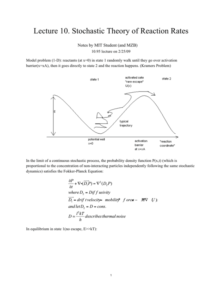
Lecture 10. Stochastic Theory of Reaction Rates Notes by MIT Student (and MZB)
10.95 lecture on 2/25/09
Model problem (1-D): reactants (at x=0) in state 1 randomly walk until they go over activation
barrier(x=xA), then it goes directly to state 2 and the reaction happens. (Kramers Problem)
In the limit of a continuous stochastic process, the probability density function P(x,t) (which is
proportional to the concentration of non-interacting particles independently following the same stochastic
dynamics) satisfies the Fokker-Planck Equation:
In equilibrium in state 1(no escape, E>>kT):
1
(Note that a Boltzmann distribution must describe the equilibrium state of zero flux, since the particles re
assumed to be non-interacting point particles .) For P(x,t), we can almost guess it would be as below:
For the 1d Kramers Problem, we consider the following initial value problem
which describes a particle released from the origin at t=o and diffusing in the energy landscape U(x). To
calculate conveniently, we put them into Dimensionless form:
Recall that the probability density function P can be interpreted as the concentration (mean number) of
non-interacting random walkers starting at x=o at t=o and arriving at
The "first passage time" T is a random variable, whose value is the time when the stochastic process
first achieves a certain condition, such as hitting a target set. In Kramers problem, this target is the
activation barrier, and <T> = mean first passage time starting from the potential welll = inverse of the
mean reaction rate. If we want complete information about fluctuations in the reaction rate (not just its
mean), we need to solve for PDF (probability density function) f(t) for T. This can be conveniently
calculated from the "survival probability" 5(t)= Probability the process has not hit the target set (here,
the activation barrier) at x=xA up to time t.
2
=Probability
(Escape
Time
>
t)
To obtain 5(t) for a general stochastic process, we solve the Fokker-Planck equation solve (l) with initial
condition localized on the starting point (2) subject to the boundary condition P=o on the target set. This
describes an "absorbing boundary" that "eats" stochastic trajectories as soon as they reach it, leaving
behind only trajectories that have "survived" and not yet hit the set. For the ld Kramers problem:
5o we get: Consider (l)'s dimensionless form into another form for next step: We will solve this problem in more general form and apply it to Kramers problem in the next lecture. 3
MIT OpenCourseWare
http://ocw.mit.edu
10.626 Electrochemical Energy Systems
Spring 2014
For information about citing these materials or our Terms of Use, visit: http://ocw.mit.edu/terms.