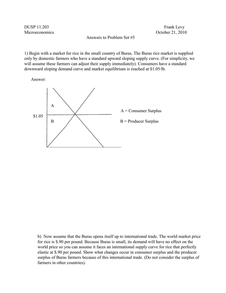
DUSP 11.203
Microeconomics
Frank Levy
October 21, 2010
Answers to Problem Set #5
1) Begin with a market for rice in the small country of Buras. The Buras rice market is supplied
only by domestic farmers who have a standard upward sloping supply curve. (For simplicity, we
will assume these farmers can adjust their supply immediately). Consumers have a standard
downward sloping demand curve and market equilibrium is reached at $1.05/lb.
Answer:
A
A = Consumer Surplus
$1.05
B
B = Producer Surplus
b) Now assume that the Buras opens itself up to international trade. The world market price
for rice is $.90 per pound. Because Buras is small, its demand will have no effect on the
world price so you can assume it faces an international supply curve for rice that perfectly
elastic at $.90 per pound. Show what changes occur in consumer surplus and the producer
surplus of Buras farmers because of this international trade. (Do not consider the surplus of
farmers in other countries).
2
A
original equilibrium
equilibrium with imports
$1.05
C
D
$.90
B
Answer: The import market means the supply curve for rice becomes perfectly elastic at $.90 – i.e.
consumers can buy as much rice as they want at $.90 cents a pound so the new equilibrium is now
where the demand curve = $.90. Given this possibility, these are the changes:
Before Imports (P = $1.05)
Consumer Surplus
Domestic Producer Surplus
A
After Imports ( P = $.90)
A+C+D
B+C
B
c) Bowing to the protests of Buras rice farmers, the government imposes a $.15 per pound tariff
on imported rice so that each pound of imported rice has $.15 added to its price. Using
appropriate diagrams show what changes this tariff makes in the consumer surplus and Buras
farmers’ producer surplus you had in (b). Can you identify the tariff revenue in your graph? If
so, how should that be counted?
Answer: I MADE A MISTAKE IN WRITING UP THIS QUESTION. I had meant to Let the
tariff to $.10 in which case the graph would have looked like the drawing below. In that
drawing, the area D is the tariff revenue which should be counted as a benefit along with
consumer and producer surplus while C, G and E are deadweight loss.
3
Original equilibrium
$1.05
A
Equilibrium with trade and tariff
G
$1.00
B
C
D
E
Equilibrium with trade but no tarriff
$.90
F
With Trade but no Tariff
Consumer Surplus
With Trade and Tariff
A+G+B+C+D+E
Domestic Producer Surplus
F
Tariff Revenue
-
A+G
F+B
D
(C and E are deadweight losses due to imposition of the tariff. In other words, they are lost from
consumer surplus but don’t become either parts of domestic producer surplus or tariff revenue.
2) NOTE: This problem involves very simple marginal and average costs curves that don’t
have the standard “U” shape so that you can work the problem in algebra.
The Cape Cod National Seashore District is about to open a new park, Tranquility Beach. District
officials want food to be sold at the beach but are unsure of how best to organize sales. Initially, the
officials decide that the only food to be sold on the beach is fried clams rolls produced in small,
tasteful clam shops. The state has done a study of clam shops and determined that their cost
structure is:
Av. Cost/Clam Roll = Marginal Cost/Clam Roll = $2.00/Clam Roll.
Both AC and MC are constant for all levels of output up to 200 clam rolls per day, the capacity of a
small tasteful clam shop.
4
The state has also done a market analysis and finds that the total demand for clam rolls from all
beach goers can be written as:
P = $10.00 - .002Q
Where P is the price per clam roll
Q is the number of clam rolls sold per day.
a) Using the information above, draw the average and marginal cost curves of a traditional clam
shop.
Answer (see graph below) AC = MC = a constant $2.00 per clam roll. (Because Average Cost is a
constant $2.00, $2.00 is also the value of minimum average cost.)
b) Suppose anyone can open a clam shop on the beach. What will be the equilibrium price of clam
rolls, the profit per shop and the total number of clam rolls sold per day?
Answer: (see graph below): This is a case of perfect competition where clam shops will keep
entering the industry until clam shops in the industry are breaking even. To calculate the answers,
begin with the fact that breaking even means Price = Average Cost = $2.00.
So we know from the outset that equilibrium price = $2.00 and profit per shop will be zero since
they are all breaking even.
To calculate the number of clam rolls per day, we can plug the $2.00 into the industry demand
curve:
$2.00 = $10.00 - .002Q or .002Q = $8.00 or Q = 4000 clam rolls sold per day.
c) After several months the state decides Tranquility Beach looks too commercial. To remedy the
situation, it announces that only four tasteful clam shops will be allowed to operate and the rest of
the shops will have to close. The four lucky shops will be chosen by lottery and as before, each shop
will be able to produce no more than 200 clam rolls per day. Assuming the shops do not cooperate
with each other and act as price takers, what will be the equilibrium price of clam rolls, the profit
per shop and the total number of clam rolls sold per day?
Answer: (see graph below). If only four shops are allowed to produce 200 clam rolls apiece, we
know that 800 clam rolls will be sold per day and the industry supply curve will be perfectly
inelastic at 800 clam rolls. (The supply curve would not look like this if the price of a clam roll fell
below $2.00 but with so few clam rolls on the market, we can be pretty sure the price will not fall
that low.)
To determine the equilibrium price, substitute 800 clam rolls into the demand curve:
P = $10.00 - .002*800 = $10.00 – $1.60 = $8.40 per clam roll.
Profit per shop = 200*($8.40 - $2.00)
profit per shop.
(i.e. quantity multiplied by (price – average cost) = $1,280
d) A few months later Citizens for Good Snacks (CGS) writes the state legislature to complain that
by limiting the number of shops and the number of clam rolls, the state has totally mismanaged
food sales on Tranquility Beach. "Believe it or not," they argue, "if the state let one of these shops
run clam roll sales as a pure monopoly without a 200 clam roll limit, consumers would be better off
than they are with the current situation."
Explain why you agree or disagree with the CGS statement. Assume in your answer that the
5
monopoly firm would retain the same cost structure with AC = MC = $2.00 per clam roll at any
level of output.
Answer: (see graph below). If one shop ran the market as a monopoly with no 200 limit on
production, they would choose output by setting marginal revenue = marginal cost.
We know MC = a constant $2.00. Because the market has a straight line demand curve, we know
that Marginal Revenue = $10.00 - .004Q (i.e. MR is also straight line with the same intercept and
twice the slope).
MR = MC means: $10.00 - .004Q = $2.00 or .004Q = $8.00 or Q = 2000 clam rolls per day, the
profit maximizing output for a monopolist.
This is really all the information we need to conclude that the CGS statement is correct. A
monopolist would produce 2000 clam rolls per day, more than twice as much as the 800 clam rolls
per day produced under the four shop limit (c). We know, without doing any calculations, that
selling 2,000 clam rolls per day will mean a lower price than selling 800 clam rolls per day so
consumers will be better off under the monopoly than under the four clam shop limit.
It is worth a minute to consider what this means. In class, we said that a monopolist restricts
output below the perfectly competitive output in order to increase profit. In (c) officials further
restricted output below the monopoly output. If you do the calculations, you will see that total
profit with four clam shops is less than total profit under the monopolist but officials were not
looking to maximize profit. Rather, they wanted to establish a particular design for how the beach
should look.
4 clam shop solution
Monopoly Solution
Perfect Competition solution
MC = AC = a constant $2.00
6
3) In the Aroostock Country, farmers produce green beans in a perfectly competitive industry. All
farms have identical technologies with these characteristics:
- A standard "U-shaped" average cost curve, etc.
- Minimum average cost is $.50 per pound of beans which occurs at an output of
1000 pounds of beans.
- The farms are all small and no farm can produce more than 2000 pounds of
beans.
The Aroostock agricultural extension service is experimenting with a new bean seed which may
be more productive than seeds now in use. To give the new seeds a fair test, the county
government runs an experiment in which it distributes unmarked packages of seeds to all farmers
now in the industry. Ninety percent of the farmers will get the old seeds. Ten percent of the
farmers will get only new seeds. If the new seeds work, they will reduce a farm's average and
marginal cost curves by exactly $.10 cents per pound at every point on each curve.
a) Using side-by-side diagrams draw the short run equilibrium for a typical green bean farm and
for the green bean industry before the experiment. In your drawings, include as much detail as the
information permits and explain how you are defining short run.
Answer: for the typical farm, P = MC = min AC at $.50 per pound which occurs at Q = 1,000 lbs.
Industry has long run flat supply curve (= minimum AC of firms = $.50/lb) up to equilibrium
point and then upward sloping after that reflecting the sum of the MC curves of firms currently in
the industry. By short run, we mean that no firms have a chance to enter or leave the industry.
b) (15 points) Assuming the seeds work, use drawings to show how the experiment will change
your short-run equilibrium in (a) for: (i) a farmer who gets the old seeds (ii) a farmer who gets
the new seeds and (iii) the green bean industry.
Answer: This is a simple version of perfect competition where different firms have different cost
curves. The firms with the new seeds will have somewhat lower cost curves. See curves below:
New Seeds
Old Seeds
Industry
7
As you can see, farms with the new seeds will have lower cost curves. They (like all farmers)
will set P = MC to maximize profits. That means they will be producing a little more than they
had produced before but since the increase is small and only 5% of the farms get the new seeds,
we can say, roughly that industry supply doesn’t change. So price stays the same at $.50/lb = min
AC of the 95% of firms that have the old seeds. New firms make a profit, old firms break even as
before.
c) (12 points) Suppose that the seeds do not work as planned and, in fact produce no green beans
at all. Using words and illustrations where appropriate, briefly describe the short run effect on (i)
a farmer who gets the old seeds (ii) a farmer who gets the new seeds and (iii) the green bean
industry.
Answer: Short run effects: farmers who get the new seeds produce nothing so they go out of
business. Since they are not producing anything, industry supply has now shrunk by roughly 5
percent. The industry supply curve moves in and so prices rise. Farms with old seeds see higher
price and make a profit (new P = MC) at least until the longer run when other firms can enter.
Old Seeds
Industry
(As shown in the graph, industry supply curve moves in because farms with the new seeds are
now producing nothing. The price rises correspondingly.
4) New York City strictly limits the number of taxi cabs on the street by requiring that each cab
have an official medallion and the city government controls the supply of medallions. In other
cities – e.g. Washington, DC - essentially anyone who wants to operate a licensed taxi can do so
by paying a modest fee to the city’s taxi bureau. In other words, in DC, entry into the industry is
very easy and so the industry is highly competitive.
Assume that DC has a standard downward sloping demand curve for taxi rides with both an
elastic and an inelastic range. To simplify the analysis, let us assume that all taxi cab rides charge
the same price regardless of distance, and that the price is determined by supply and demand.
a) In general terms, describe the main factors that will determine the long run equilibrium price of
a taxicab ride in DC
Answer: Assume that all cabs have similar costs curves. Since entry of new cabs into the industry
is very easy, we would expect the price of a cab ride to decline to the point where the price =
minimum average cost of the typical cab and all cabs will be breaking even.
8
If you want to get fancy and assume that cabs have different costs, then the price will equal the
minimum average cost of the least efficient cab in the is in the industry and all other cabs will
make profits (rents) that go to the factor that is causing their cost curves to be lower – e.g. more
skilled drivers, etc. The bottom line is that it is the cost curve of either the typical cab (identical
technologies) or the marginal cab (different technologies) that determines the long run equilibrium
price.
b) Explain whether this DC equilibrium price will occur on the elastic portion of the demand
curve or the inelastic portion of the demand curve. If you do not have enough information to
answer the question, explain why
Answer: We don’t have enough information. We know from (a) that entry forces the price down
to the minimum average cost of a cab. There is no particular connection between the cost curves
of the cab and the shape of the demand curve – i.e. where it is elastic or inelastic.
c) Suppose, instead, that the DC city government decides to run the taxicab industry as a
monopoly, limiting the number of cabs to produce the profit maximizing number of rides for the
industry. Will the resulting price lie on the elastic or inelastic portion of the demand curve for
taxicab rides? Explain. If you do you not have enough information to answer the question,
explain why.
Answer: This is an example of a more general idea: A monopolist can never maximize profit on
the inelastic portion of the demand curve. We can show this by looking at formulae or by using
common sense. Using formulae, we know profit maximization occurs where MR = MC. We also
know that the inelastic portion of a demand curve corresponds to negative marginal revenue.
Negative marginal cost is basically impossible (it would mean that producing more units would
reduce TOTAL cost) so MR = MC won’t happen at a quantity where the demand curve is
inelastic.
The common sense argument goes like this. Suppose a monopolist is producing output on an
inelastic portion of the demand curve. She knows that if she cuts back quantity on an inelastic
portion of the demand curve (i.e. raising her price) Total Revenue will increase. She also can
assume that is she cuts back on quantity, her Total Cost will decrease. Put these effects together
and they indicate that if she cuts back quantity profits will improve. In other words, if she is on an
inelastic portion of the demand curve, she can always improve profits by reducing the quantity
produced (which means moving back toward the elastic portion of the demand curve.)
***************************************************
MIT OpenCourseWare
http://ocw.mit.edu
11.203 Microeconomics
Fall 2010
For information about citing these materials or our Terms of Use, visit: http://ocw.mit.edu/terms.