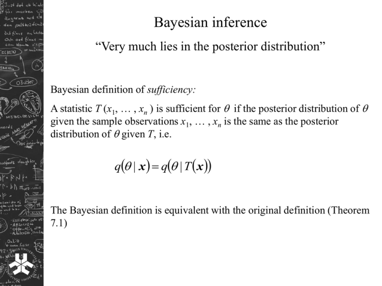
Bayesian inference
“Very much lies in the posterior distribution”
Bayesian definition of sufficiency:
A statistic T (x1, … , xn ) is sufficient for  if the posterior distribution of 
given the sample observations x1, … , xn is the same as the posterior
distribution of  given T, i.e.
q | x   q | T  x 
The Bayesian definition is equivalent with the original definition (Theorem
7.1)
Credible regions
Let  be the parameter space for  and let Sx be a subset of .
If
 qθ | x dθ  1  
Sx
then Sx is a 1 –  credible region for  .
For  a scalar we refer to it as a credible interval
The important difference compared to confidence regions:
A credible region is a fixed region (conditional on the sample) to which
the random variable  belongs with probability 1 – .
A confidence region is a random region that covers the fixed  with
probability 1 – 
Highest posterior density (HPD) regions
If for all θ1  S x , θ2  S x
qθ1 | x   qθ2 | x 
then S x is called a 1   highest posterior density (HPD) credible region
Equal-tailed credible intervals
An equal-tailed 1 –  credible interval is a 1 –  credible interval (a , b )
such that
Pr  a | x   Pr  b | x    2
Example:
In a consignment of 5000 pills suspected to contain the drug Ecstasy a
sample of 10 pills are sampled for chemical analysis. Let  be the
unknown proportion of Ecstasy pills in the consignment and assume we
have a high prior belief that this proportion is 100%.
Such a high prior belief can be modelled with a Beta density
  1 1    1
p   
B  ,  
where  is set to 1 and  is set to a fairly high value, say 20, i.e. Beta
(20,1)
Beta(20,1)

0
0.2
0.4
0.6
0.8
1
Now, suppose after chemical analysis of the 10 pills, all of them showed
to contain Ecstasy.
The posterior density for  is Beta( + x,  + n – x) (conjugate prior
with binomial sample distribution as the population is large)

Beta (20 + 10, 1 + 10 – 10) = Beta (30, 1)
Then a lower-tail 99% credible interval for  satisfies
1
x 29
 B30,1dx  0.99
a



1
 1  a 30  0.99
30 B30,1
 a  1  0.99  30 B30,11 30  0.858
Thus with 99% certainty we can state that at least 85.8% of the pills in the
consignment consist of Ecstasy
Comments:
We have used the binomial distribution for the sample. More correct
would be to use the hypergeometric distribution, but the binomial is a
good approximation.
For a smaller consignment (i.e. population) we can benefit on using the
result that the posterior for the number of pills containing Ecstasy in the
rest of the consignment after removing the sample is beta-binomial.
This would however give similar results
If a sample consists of 100% of one kind, how would a confidence
interval for  be obtained?
Bayesian hypothesis testing
The issue is to test H0 vs. H1
Without specifying the hypotheses further, we seek to judge upon which
of the two hypothesis that, conditional on the sample, is the most
probable.
Note the difference compared to the classical approach: There we seek to
reject H0 in favour of H1 and never the opposite.
The aim of Bayesian hypothesis testing is to determine the posterior
“odds”
Q* 
Pr H 0 | x 
Pr H1 | x 
With Q* > 1 we then say that conditional on the sample H0 is Q* times
more probable than H1 and with Q* < 1 the expression is reversed.
Some review of probability theory:
For two events A and B from a random experiment we have
Pr  A | B  
Pr B | A Pr  A
Pr B 

Pr B | A Pr  A
Pr  A | B 
Pr B | A Pr  A
Pr B 



Pr A | B
Pr B | A Pr A
Pr B | A Pr A
Pr B 



 

 
Actually A can be replaced by any other event C , but when
A is used the relation can be written
Pr B | A
Odds  A | B  
 Odds  A
Pr B | A


This result is usually referred to as Bayes theorem on odds form
Now, it is possible to replace A with H0 , A with H1 and B with x (the
sample)

Pr H 0 | x  f  x | H 0  Pr H 0 


Pr H1 | x  f  x | H1  Pr H1 

Q* 
f x | H0 
Q
f  x | H1 
where Q is the prior “odds”
Note that
f x | H0 
LH 0 ; x 
can sometimes be written
f  x | H1 
L  H1 ; x 
where L(H ; x) is the likelihood of H . The concept of likelihood is not
restricted to parameters.
Note also that f (x | H0) need not have the same functional form as
f (x | H1)
f x | H0 
B
will be referred to as the Bayes factor
f  x | H1 
(and is sometimes a likelihood ratio)
To make the comparison with classical hypothesis testing more
transparent the posterior odds may be transformed to posterior
probabilities for each of the two hypotheses:
Pr H 0 | x  
Pr H1 | x  
Q*
Q*  1
1
Q*  1
Now, if the posterior probability of H1 is 0.95 this would be a result that
could be compared with “H0 is rejected at 5% level of significance”
However, the two approaches cannot be made equal
Another example from forensic science
Assume a crime has been conducted where a blood stain was left at the
crime scene. A suspect is identified and a saliva sample is taken from this
person. The DNA profiles are compared between the saliva sample and the
blood stain and they appear to match (i.e. they are equal).
Put
H0: “The blood stain comes from the suspect”
H1: “The blood stain comes from another person than the suspect
The Bayes factor becomes
B
Pr Matching DNA profiles | H 0 
Pr Matching DNA profiles | H1 
Now, if laboratory mistakes can be discarded
Pr (Matching DNA profiles | H0 ) = 1
How about the probability in the denominator of B ?
This probability relates to the commonness of the current profile among
people in general.
Today’s DNA analysis is such that if a full profile is obtained (i.e. if there
are no missing DNA markers), the probability is very low, about 1 in 10
million.
 B becomes very large
If the suspect was caught on reasons not related to the DNA-analysis (as
it should be), the prior odds, Q = Pr (H0 ) / Pr (H1 ) is probably greater
than 1
If we calculate with Q =1 then Q* = B and thus very large
 The DNA analysis very strongly supports H0 to be true.
Hypotheses expressed in terms of a parameter
For sake of simplicity we express the parameter as a scalar, but the results
also apply to multidimensional parameters 
Case 1: H0:  = 0
H1:  = 1
Pr H 0   p0 ; Pr H1   p1 ; B 
f  x; 0 
f  x;1 
Example: Let x be an observation from Bin(n,  ) and
H0:  = 0 vs. H1:  = 1

Q
p0
p1
n x
   0 1   0 n x
x
n x
x





1  0

; B 
  0  

1  1 
n x
  1 1   1 n x  1  
 x
 
 Q*   0 
 1 
x
1  0 


 1  1 
n x
p0
p1
Case 2: H0:   
Pr H 0  
Pr H1  
H1:    –  ( \  )
 p0  H 0 d   p0  H 0 d ;
H0



H1
p1  H1 d 
 
 f  x;  p0  H 0 d
B 
 f  x;  p1  H1 d
 
 d ;
p1 
L1
Case 3: H0:  = 0
H1:   0
Pr H 0   p0  0  ; Pr H1  
 p1  H1 d   p1  H1 d
H1
B
  0
f  x; 0 
 f  x;  p1  H1 d
  0
It can be shown (Theorem 7.3) that in this case
q | x 
  0 p 
B  lim
(As   0 defines the region for H1 the conditioning on H1 in the
textbook seems redundant. )
Nuisance parameters and predictive distributions
If the parameters involved are two  and  and the parameter of interest is
, then  is referred to as a nuisance parameter.
The marginal posterior density for  is then obtained by integrating out 
from the joint posterior density:
qθ | x    qθ , λ | x  dλ

where  is the parameter space for .
Predictive distributions
Let xn = ( x1, … , xn ) be a random sample from a distribution with p.d.f. f
(x ;  )
Suppose we will take a new observation xn + 1 and would like to make socalled predictive inference about it. In practice this means that we would
like to express the uncertainty about it in terms of a prediction interval.
The marginal p.d.f. of Xn + 1 is the same as that of each variable Xi in the
sample, i.e. f (x ;  )
However, if we want to make use of the sample we should rather study the
simultaneous density of Xn + 1 and  | xn .
Xn + 1 and Xn are independent by definition
 Xn + 1 and  | xn are also independent as the latter is conditional on xn
The simultaneous density of Xn + 1 and  | x is
f xn1; θ   qθ | xn 
Now, treating  (temporarily) as a nuisance parameter.
The posterior predictive distribution (density) for Xn + 1 given  and xn is
then
g  xn1 | xn  
 f xn1; θ  qθ | xn dθ

g can be used to
• find a point prediction of Xn + 1 as
– the mean of g with quadratic loss, i.e.  t  g t | xn dt
R1
– the median of g with absolute error loss
– the mode of g with zero-one loss
• compute a 1 –  prediction interval for Xn + 1 by solving for c and d
c g t | xn dt  1  
d
usually w ith equal tails
Example
The number of calls to a telephone central during an hour can usually be
shown to follow a Poisson distribution with mean . Assume that a prior
for  is a Gamma (a,b)-distribution, i.e. the prior density is
b a 1a e b
p  
a  1
Now assume that we have observed x1, x2 and x3 calls during each of the
three previous hours and we wish to make predictive inference about the
number of calls x4 during the current hour.
The posterior distribution is also Gamma with

b  3a  x  x  x 1 a  x  x  x e  b 3
q | x1 , x2 , x3  
a  x1  x2  x3  1
b  3at 1 at e b3

a  t  1
1
with t  x1  x2  x3
2
3
1
2
3

Now,
a  t 1 a  t  b  3


b

3
 e
g  x4 | x1 , x2 , x3   
e 
d 
x !
a  t  1
0 4

x
4
b  3at 1 a t  x4 e b 4 
1


d 
x4 ! 0
a  t  1

1 a  t  x4  1 b  3a  t 1




a

t

x

1
4
x4 !
a  t  1
b  4

b  4a t  x4 1 a  t  x4 e b 4 
 
d 
a  t  x4  1
0

 1 (Gamma density)
 b3


b 4
a  t 1

1
1

a  t  1 b  4 x4 x4!
and e.g. a point prediction under quadratic loss of the number of
calls is obtained by

 b3
 x   b  4 
x0
a  t 1
1
1



x
a  t  1 b  4  x!
 b3


b 4
a  t 1


1
1 b  4 x

x


a  t  1 x  0
x!
 b3


b 4
a  t 1
x





1
1
b

4

 e1 b 4   x 
 e 1 b 4  
a  t  1
! 

x  0 x
p.m.f. of Po 1 b  4 
 b3


b 4
a  t 1

1
1
 e1 b 4  
a  t  1
b4
Empirical Bayes
“Something between the Bayesian and the frequentist approach”
General idea:
Use some of the available data (sample) to estimate the prior for 
Use the rest of the available data to make inference about 
Parametric set-up:
Let data-point i be represented by the bivariate random variable (Xi , i ),
i =1, 2, …, k
Let f (x; i ) be the p.d.f. for Xi and p( ) be the marginal density of i
f is assumed to be known part from  and p is assumed to be unknown.
1, … , k are unobservable quantities.
With Empirical Bayes we try to make inference about k
Use x1, … , xk – 1 to estimate p( )
Then make inference about k through its posterior distribution
conditional on xk
f xk ; k  pˆ  k 
q k | xk  
 f xk ;  pˆ  d
the usual way:
• point estimation under certain choices of loss functions
• credible regions
• hypothesis testing
How to estimate p( ) ?
The marginal density for Xi is f x    f x;  p d
Let p = p( ; ) where  is a (multidimensional) parameter defining the
prior assuming the functional form of p is known.
Method of moments:
Put up the equations
 xf x dx E  X   Eψ E  X |      xf x; dxp ; ψ d
Var  X   Eψ Var  X |   Varψ E  X |  
from which an estimate of  can be deduced.
Maximum-Likelihood:
 is estimated as
k 1
ψˆ  arg max Lψ; x1,, xk 1   
ψ
i 1
 f xi ;  p ; ψ d 
Apparently, the textbook is not correct here as the estimation of p should
be based on the first k – 1 observations and the kth should be excluded
from that stage.
See further the textbook for simplifications of the MLE procedure.