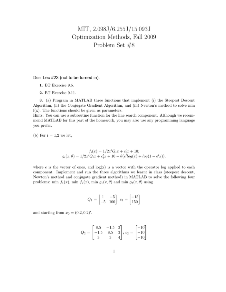
MIT, 2.098J/6.255J/15.093J
Optimization Methods, Fall 2009
Problem Set #8
Due: Lec #23 (not to be turned in).
1. BT Exercise 9.5.
2. BT Exercise 9.11.
3. (a) Program in MATLAB three functions that implement (i) the Steepest Descent
Algorithm, (ii) the Conjugate Gradient Algorithm, and (iii) Newton’s method to solve min
f(x). The functions should be given as parameters.
Hints: You can use a subroutine function for the line search component. Although we recom­
mend MATLAB for this part of the homework, you may also use any programming language
you prefer.
(b) For i = 1,2 we let,
gi (x, θ) =
fi (x) = 1/2x′ Qi x + c′i x + 10;
′
1/2x Qi x + c′i x + 10 − θ(e′ log(x) +
log(1 − e′ x)),
where e is the vector of ones, and log(x) is a vector with the operator log applied to each
component. Implement and run the three algorithms we learnt in class (steepest descent,
Newton’s method and conjugate gradient method) in MATLAB to solve the following four
problems: min f1 (x), min f2 (x), min g1 (x, θ) and min g2 (x, θ) using
�
�
�
�
1 −5
−15
Q1 =
; c1 =
−5 100
150
and starting from x0 = (0.2, 0.2)′ .




8.5 −1.5 3
−10
Q2 = −1.5 8.5 3; c2 = −10
3
3
4
−10
1
and starting from x0 = (0.3, 0.4, 0.1)′ and θ = 1.
(c) For each of the three algorithms, plot f (xk ) vs. k and
is the optimal solution.
f (xk+1 )−f (x∗ )
f (xk )−f (x∗ )
vs k, where x∗
(d) Using the answer to (c), discuss the rate of convergence for each of the three algo­
rithms and compare it with the one predicted from theory.
(e) Illustrate numerically what happens to the solution of the problem min g2 (x, θ) as θ
varies in the interval [0.01, 10].
4. Consider the following problem:
min
s.t.
f (x) = −x1
x21 + x22 ≤ 1
(x1 − 1)3 − x2 ≤ 0
• Show that the KKT constraint qualification holds at point x = (1, 0).
• Show that point x = (1, 0) is a KKT point and also a global optimal solution.
5. (a) Use the KKT conditions to solve the following problem
min
s.t.
f (x) = x′ Qx + c′ x
g(x) = x′ Rx ≤ 1
e′ x = 1
where Q is an invertible matrix, although not necessarily positive definite and R is a positive
definite matrix. Note that e is a vector of ones.
(b) Apply your solution to the case where


 


1 0 −2
−1
1
−0.5 −0.4
Q2 =  0 1 0 ; c2 = −1; R = −0.5
1
0 ;
−2 0 1
−1
−0.4
0
1
2
MIT OpenCourseWare
http://ocw.mit.edu
15.093J / 6.255J Optimization Methods
Fall 2009
For information about citing these materials or our Terms of Use, visit: http://ocw.mit.edu/terms.
-
1