15.075 Statistical Thinking and Data Analysis
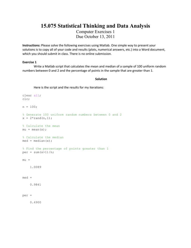
Computer Exercises 1 Due October 13, 2011 Instructions: Please solve the following exercises using Matlab. One simple way to present your solutions is to copy all of your code and results (plots, numerical answers, etc.) into a Word document, which you should submit in class. There is no online submission. Exercise 1 Write a Matlab script that calculates the mean and median of a sample of 100 uniform random numbers between 0 and 2 and the percentage of points in the sample that are greater than 1. Solution Here is the script and the results for my iterations: clear all;
clc;
n = 100;
% Generate 100 uniform random numbers between 0 and 2
x = 2*rand(n,1);
% Calculate the mean
mu = mean(x);
% Calculate the median
med = median(x);
% Find the percentage of points greater than 1
per = sum(x>1)/n; mu =
1.0089
med =
0.9841
per =
0.4900
Exercise 2 a. Generate a vector of 1000 normal random numbers with mean 8 and variance 25. b. Calculate how many elements in the vector are greater than or equal to 9. c. What is the sample mean and standard deviation for this sample of 1000 numbers? d. What are the 25th and 75th percentiles of the normal distribution with mean 8 and variance 25? e. What are the 25th and 75th percentiles of the sample of the 1000 normal random numbers generated in part (a)? f. Find Φ(0.789) and Φ(‐0.543). (Remember Φ is the cumulative density function for the standard normal distribution.) Solution Here is the script and the results for my iterations: clear all;
clc;
n = 1000;
mu = 8;
sigma = 5;
% a.
Generate a vector of 1000 normal random numbers with mean 8 and
variance 25.
x = sigma*randn(n,1)+mu;
% b.
Calculate how many elements in the vector are greater than or equal
to 9.
num = sum(x>=9)
% c.
What is the sample mean and standard deviation for this sample of
1000 numbers?
sample_mean = mean(x)
sample_std = std(x)
% d.
What are the 25th and 75th percentiles of the normal distribution
with mean 8 and variance 25?
q1 = norminv(.25,8,5) % or q1 = 5*norminv(0.25)+8
q3 = norminv(.75,8,5) % or q1 = 5*norminv(0.75)+8
% e.
What are the 25th and 75th percentiles of the sample of the 1000
normal random numbers generated in part (a)?
s_q1 = quantile(x,0.25)
s_q3 = quantile(x,0.75)
% f.
Find ?(0.789) and ?(-0.543).
normcdf(0.789)
normcdf(-0.543) num =
428
sample_mean =
8.0511 sample_std =
4.9974
q1 =
4.6276
q3 =
11.3724
s_q1 =
4.7150
s_q3 =
11.2380
ans =
0.7849
ans =
0.2936
Exercise 3 a. Generate a vector of 1000 Poisson random numbers with λ = 2. b. Make a histogram and a boxplot of the 1000 numbers from part (a). Solution Here is the script and the plots for my iterations:
clear all;
clc;
close all;
n = 1000;
lambda = 2;
% a.
Generate a vector of 1000 Poisson random numbers with ? = 2.
x = poissrnd(lambda,n,1);
% b.
Make a histogram and a boxplot of the 1000 numbers from part (a).
figure;
hist(x);
figure;
boxplot(x);
Exercise 4 Answer questions (a) – (c) from 4.36 in your textbook. Solution Here is the script and a scatterplot:
clear all;
close all;
clc;
snowfall = [45 59 82 80 71 60 55 69 79 95];
unemployment = [4.9 5.6 8.5 7.7 7.1 6.1 5.8 7.1 7.6 9.7];
% Scatterplot
plot(snowfall, unemployment, 'x');
grid;
xlabel('Snowfall (inches)');
ylabel('Unemployment (%)');
% Calculates the correlation coefficient
rho = corr(snowfall',unemployment'); rho = 0.9835 A strong linear positive relationship is indicated by both the scatter plot and the correlation coefficient. This relationship does not mean that the snowfall influences the national unemployment rates or vice versa. It means that there is an association between them. 4.44
a.
Below is a time-series plot of the data. There is an increasing trend, so no, the time-series does
not appear to be stationary.
159
160
161
CPI
162
163
164
CPI for 1997−1998
5
10
15
20
Month/Year
b,c. The moving averages and exponentially weighted moving averages are listed below. The MAPE
is 0.2655% and 0.5679% for MA and EWMA respectively.
MA
159.1000
159.3500
159.5667
159.9333
160.1000
160.2000
160.3000
160.5333
160.8333
EWMA
159.1000
159.2000
159.3600
159.5280
159.6424
159.7739
159.9191
160.0953
160.3162
2
161.2000
161.4333
161.4667
161.4667
161.6000
161.9000
162.2000
162.5000
162.7667
163.0000
163.2000
163.4000
163.6667
163.8667
163.9667
160.5730
160.7584
160.8667
161.0134
161.1907
161.3926
161.6140
161.8512
162.0810
162.3048
162.5238
162.7391
162.9913
163.1930
163.3344
d. We have r1 = 0.8694, r2 = 0.7380, and r3 = 0.6149. So CPI in successive months have a rather
strong positive correlation, but the correlation grows weaker with CPI’s removed farther apart.
3
MIT OpenCourseWare
http://ocw.mit.edu
15.075J / ESD.07J Statistical Thinking and Data Analysis
Fall 2011
For information about citing these materials or our Terms of Use, visit: http://ocw.mit.edu/terms.