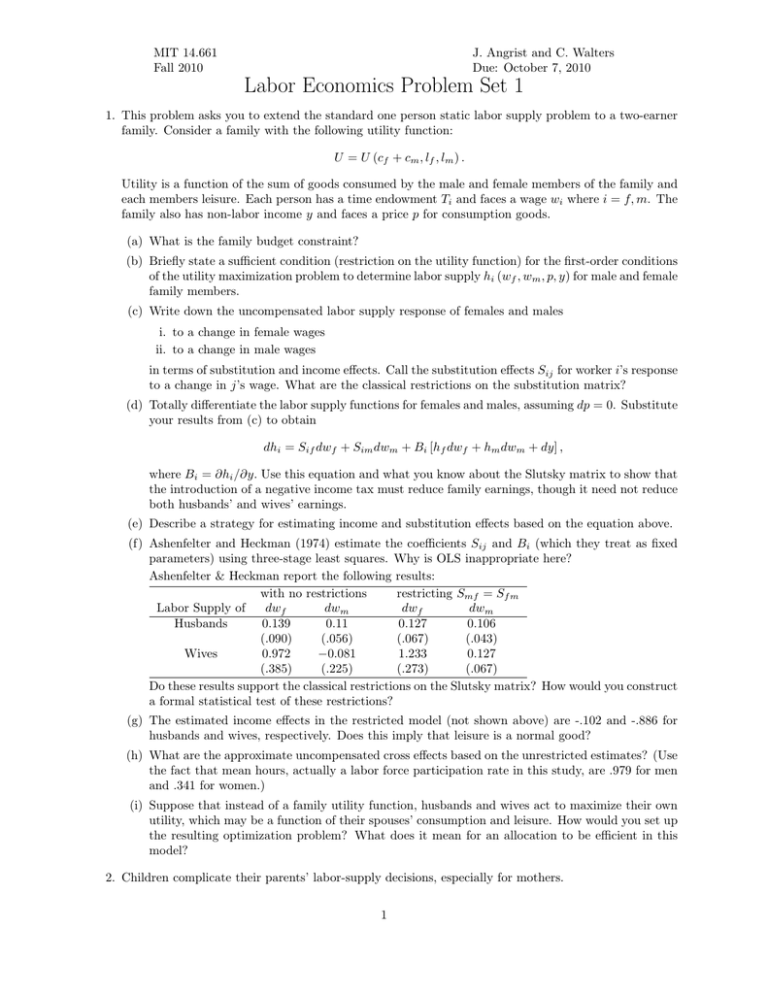
MIT 14.661
Fall 2010
J. Angrist and C. Walters
Due: October 7, 2010
Labor Economics Problem Set 1
1. This problem asks you to extend the standard one person static labor supply problem to a two-earner
family. Consider a family with the following utility function:
U = U (cf + cm , lf , lm ) .
Utility is a function of the sum of goods consumed by the male and female members of the family and
each members leisure. Each person has a time endowment Ti and faces a wage wi where i = f, m. The
family also has non-labor income y and faces a price p for consumption goods.
(a) What is the family budget constraint?
(b) Briefly state a sufficient condition (restriction on the utility function) for the first-order conditions
of the utility maximization problem to determine labor supply hi (wf , wm , p, y) for male and female
family members.
(c) Write down the uncompensated labor supply response of females and males
i. to a change in female wages
ii. to a change in male wages
in terms of substitution and income effects. Call the substitution effects Sij for worker i’s response
to a change in j’s wage. What are the classical restrictions on the substitution matrix?
(d) Totally differentiate the labor supply functions for females and males, assuming dp = 0. Substitute
your results from (c) to obtain
dhi = Sif dwf + Sim dwm + Bi [hf dwf + hm dwm + dy] ,
where Bi = ∂hi /∂y. Use this equation and what you know about the Slutsky matrix to show that
the introduction of a negative income tax must reduce family earnings, though it need not reduce
both husbands’ and wives’ earnings.
(e) Describe a strategy for estimating income and substitution effects based on the equation above.
(f) Ashenfelter and Heckman (1974) estimate the coefficients Sij and Bi (which they treat as fixed
parameters) using three-stage least squares. Why is OLS inappropriate here?
Ashenfelter & Heckman report the following results:
with no restrictions
restricting Smf = Sf m
Labor Supply of
dwf
dwm
dwf
dwm
Husbands
0.139
0.11
0.127
0.106
(.090)
(.056)
(.067)
(.043)
Wives
0.972
−0.081
1.233
0.127
(.385)
(.225)
(.273)
(.067)
Do these results support the classical restrictions on the Slutsky matrix? How would you construct
a formal statistical test of these restrictions?
(g) The estimated income effects in the restricted model (not shown above) are -.102 and -.886 for
husbands and wives, respectively. Does this imply that leisure is a normal good?
(h) What are the approximate uncompensated cross effects based on the unrestricted estimates? (Use
the fact that mean hours, actually a labor force participation rate in this study, are .979 for men
and .341 for women.)
(i) Suppose that instead of a family utility function, husbands and wives act to maximize their own
utility, which may be a function of their spouses’ consumption and leisure. How would you set up
the resulting optimization problem? What does it mean for an allocation to be efficient in this
model?
2. Children complicate their parents’ labor-supply decisions, especially for mothers.
1
(a) Use a graph to show how women’s labor supply decisions are affected by child care costs, assuming
she is the only adult in the household.
(b) Describe the impact of a lump-sum child allowance that is phased out as income or earnings rise.
Compare this with the effect of publicly-provided child care for all, as is often found in Europe.
(c) Discuss the ways in which state-provided out-of-home care might affect children. What does the
evidence suggest?
3. Life-cycle labor supply
(a) Derive the λ-constant labor supply and commodity demand functions for the Heckman and
MaCurdy (1980) utility function. To simplify notation, use time subscripts instead of paren­
theses. You can also assume the interest rate is fixed.
i. What is the intertemporal substitution elasticity for this model? Why is this parameter
necessarily (i.e., theoretically) positive? How do wages affect consumption? Why?
ii. What does this model predict about the behavioral response to the following sources of
variation in wages: Cross-sectional variation associated with permanent differences in human
capital; Wage increases generated by changes in labor market experience; Transitory shocks
caused by changes in the macro economy; Changes in after-tax wages caused by a temporary
NIT program; Job loss at age 50.
(b) Construct a PSID extract similar to the one used by Angrist (1991). PSID data are available
from the ICPSR:
http://www.icpsr.umich.edu/cocoon/ICPSR/STUDY/07439.xml
(use the Wave I cross-year individual file).
i. Calculate the grouped-data, Analysis of Covariance (fixed-effects), and OLS estimates of
MaCurdry’s (1981) specification reported by Angrist (1991, Table 3). You should be able to
come close to these estimates after replicating the sample selection criteria and estimation
procedures as best you can.
ii. What is the Angrist (1991) interpretation of the differences in results across methods?
iii. Why does Card (1994) take a skeptical view of the large positive intertemporal substitution
elasticities that are generated by the grouped-data estimator in PSID data? Do bicycle
messengers and cab drivers answer Card’s concerns?
2
MIT OpenCourseWare
http://ocw.mit.edu
14.661 Labor Economics I
Fall 2010
For information about citing these materials or our Terms of Use, visit: http://ocw.mit.edu/terms.