6.01: Introduction to EECS I
Lecture 3
6.01: Introduction to EECS I
February 15, 2011
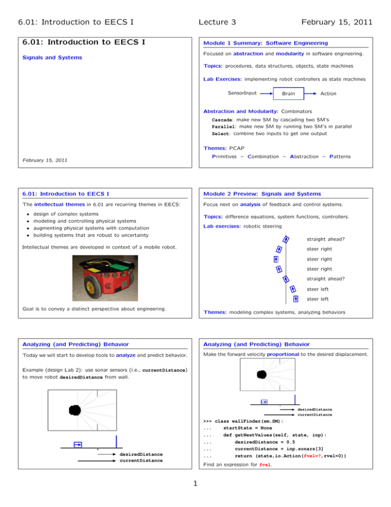
Module 1 Summary: Software Engineering
Focused on abstraction and modularity in software engineering.
Signals and Systems
Topics: procedures, data structures, objects, state machines
Lab Exercises: implementing robot controllers as state machines
SensorInput
Brain
Action
Abstraction and Modularity: Combinators
Cascade: make new SM by cascading two SM’s
Parallel: make new SM by running two SM’s in parallel
Select: combine two inputs to get one output
Themes: PCAP
Primitives – Combination – Abstraction – Patterns
February 15, 2011
6.01: Introduction to EECS I
Module 2 Preview: Signals and Systems
The intellectual themes in 6.01 are recurring themes in EECS:
Focus next on analysis of feedback and control systems.
•
•
•
•
design of complex systems
modeling and controlling physical systems
augmenting physical systems with computation
building systems that are robust to uncertainty
Topics: difference equations, system functions, controllers.
Lab exercises: robotic steering
straight ahead?
Intellectual themes are developed in context of a mobile robot.
steer right
steer right
steer right
straight ahead?
steer left
steer left
Goal is to convey a distinct perspective about engineering.
Themes: modeling complex systems, analyzing behaviors
Analyzing (and Predicting) Behavior
Analyzing (and Predicting) Behavior
Today we will start to develop tools to analyze and predict behavior.
Make the forward velocity proportional to the desired displacement.
Example (design Lab 2): use sonar sensors (i.e., currentDistance)
to move robot desiredDistance from wall.
desiredDistance
currentDistance
>>> class wallFinder(sm.SM):
...
startState = None
...
def getNextValues(self, state, inp):
...
desiredDistance = 0.5
...
currentDistance = inp.sonars[3]
...
return (state,io.Action(fvel=?,rvel=0))
desiredDistance
currentDistance
Find an expression for fvel.
1
6.01: Introduction to EECS I
Lecture 3
Check Yourself
February 15, 2011
Check Yourself
Which plot best represents currentDistance?
desiredDistance
currentDistance
1.
2.
desiredDistance
currentDistance
n
Which expression for fvel has the correct form?
n
3.
1. currentDistance
2. currentDistance-desiredDistance
3. desiredDistance
4. currentDistance/desiredDistance
4.
n
5. none of the above
n
5. none of the above
Example: Mass and Spring
Example: Tanks
r0 (t)
x(t)
h1 (t)
r1 (t)
y(t)
h2 (t)
x(t)
r0 (t)
y(t)
mass &
spring
system
t
r2 (t)
r2 (t)
tank
system
t
t
Example: Cell Phone System
t
Signals and Systems: Widely Applicable
The Signals and Systems approach has broad application: electrical,
mechanical, optical, acoustic, biological, financial, ...
sound out
x(t)
y(t)
t
mass &
spring
system
t
tank
system
sound in
t
r0 (t)
sound in
h1 (t)
sound out
t
cell
phone
system
r1 (t)
r0 (t)
h2 (t)
r2 (t)
r2 (t)
t
sound in
sound out
t
2
t
cell
phone
system
t
6.01: Introduction to EECS I
Lecture 3
February 15, 2011
Signals and Systems: Modular
Signals and Systems: Hierarchical
The representation does not depend upon the physical substrate.
Representations of component systems are easily combined.
Example: cascade of component systems
sound
in
sound out
sound in
© FreeFoto.com. CC by-nc-nd.
This content is excluded from our
Creative Commons license. For more
E/M cell
optic
cell E/M
tower
tower
phone
fiber
phone
sound
out
Composite system
sound
in
information, see http://ocw.mit.edu/fairuse.
cell phone system
sound
out
E/M cell sound
optic
sound cell E/M
tower
tower
phone
in
fiber
phone out
focuses on the flow of information, abstracts away everything else
Component and composite systems have the same form, and are
analyzed with same methods.
The Signals and Systems Abstraction
Continuous and Discrete Time
Our goal is to develop representations for systems that facilitate
analysis.
Inputs and outputs of systems can be functions of continuous time
signal
in
system
or discrete time.
signal
out
Examples:
• Does the output signal overshoot? If so, how much?
• How long does it take for the output signal to reach its final value?
We will focus on discrete-time systems.
Difference Equations
Difference Equations
Difference equations are an excellent way to represent discrete-time
systems.
Difference equations are mathematically precise and compact.
Example:
y[n] = x[n] − x[n − 1]
Example:
y[n] = x[n] − x[n − 1]
Let x[n] equal the “unit sample” signal δ[n],
�
δ[n] =
Difference equations can be applied to any discrete-time system;
they are mathematically precise and compact.
1,
0,
if n = 0;
otherwise.
x[n] = δ[n]
−1 0 1 2 3 4
n
We will use the unit sample as a “primitive” (building-block signal)
to construct more complex signals.
3
6.01: Introduction to EECS I
Lecture 3
February 15, 2011
Step-By-Step Solutions
Multiple Representations of Discrete-Time Systems
Difference equations are convenient for step-by-step analysis.
Block diagrams are useful alternative representations that highlight
visual/graphical patterns.
Find y[n] given x[n] = δ[n]:
x[n] = δ[n]
−1 0 1 2 3 4
y[n] = x[n] − x[n − 1]
Difference equation:
y[−1] = x[−1] − x[−2]
=0−0=0
y[0] = x[0] − x[−1]
=1−0=1
y[1] = x[1] − x[0]
= 0 − 1 = −1
y[2] = x[2] − x[1]
=0−0=0
y[3] = x[3] − x[2]
...
=0−0=0
y[n] = x[n] − x[n − 1]
Block diagram:
x[n]
+
−1
y[n]
Delay
y[n]
n
Same input-output behavior, different strengths/weaknesses:
• difference equations are mathematically compact
• block diagrams illustrate signal flow paths
n
−1 0 1 2 3 4
Step-By-Step Solutions
Check Yourself
Block diagrams are also useful for step-by-step analysis.
DT systems can be described by difference equations and/or
block diagrams.
Represent y[n] = x[n] − x[n − 1] with a block diagram: start “at rest”
x[n]
y[n]
+
−1
Delay
Difference equation:
y[n] = x[n] − x[n − 1]
Block diagram:
x[n]
0
+
−1
x[n] = δ[n]
y[n]
Delay
y[n]
In what ways are these representations different?
−1 0 1 2 3 4
n
−1 0 1 2 3 4
n
From Samples to Signals
From Samples to Signals
Lumping all of the (possibly infinite) samples into a single object
– the signal – simplifies its manipulation.
Operators manipulate signals rather than individual samples.
+
X
Y
−1
This lumping is analogous to
• representing coordinates in three-space as points
• representing lists of numbers as vectors in linear algebra
• creating an object in Python
Delay
Nodes represent whole signals (e.g., X and Y ).
The boxes operate on those signals:
•
•
•
Delay = shift whole signal to right 1 time step
Add = sum two signals
−1: multiply by −1
Signals are the primitives.
Operators are the means of combination.
4
6.01: Introduction to EECS I
Lecture 3
Operator Notation
February 15, 2011
Operator Notation: Check Yourself
Symbols can now compactly represent diagrams.
Let R represent the right-shift operator:
Let Y = RX. Which of the following is/are true:
Y = R{X} ≡ RX
1. y[n] = x[n] for all n
where X represents the whole input signal (x[n] for all n) and Y
represents the whole output signal (y[n] for all n)
2. y[n + 1] = x[n] for all n
3. y[n] = x[n + 1] for all n
Representing the difference machine
X
+
4. y[n − 1] = x[n] for all n
Y
5. none of the above
−1
Delay
with R leads to the equivalent representation
Y = X − RX = (1 − R) X
Operator Representation of a Cascaded System
Operator Algebra
System operations have simple operator representations.
Operator expressions expand and reduce like polynomials.
+
X
−1
Delay
Y1
+
−1
+
X
Cascade systems → multiply operator expressions.
−1
Y2
Delay
Y1
+
−1
Delay
Y2
Delay
Using difference equations:
y2 [n] = y1 [n] − y1 [n − 1]
Using operator notation:
= (x[n] − x[n − 1]) − (x[n − 1] − x[n − 2])
Y1 = (1 − R) X
= x[n] − 2x[n − 1] + x[n − 2]
Y2 = (1 − R) Y1
Using operator notation:
Substituting for Y1 :
Y2 = (1 − R) Y1 = (1 − R)(1 − R) X
Y2 = (1 − R)(1 − R) X
= (1 − R)2 X
= (1 − 2R + R2 ) X
Operator Approach
Operator Algebra
Applies your existing expertise with polynomials to understand block
diagrams, and thereby understand systems.
Operator notation facilitates seeing relations among systems.
“Equivalent” block diagrams (assuming both initially at rest):
+
X
−1
+
−1
Delay
+
X
Delay
−2
Delay
Equivalent operator expression:
(1 − R)(1 − R) = 1 − 2R + R2
5
Y1
Delay
Y
Y2
6.01: Introduction to EECS I
Lecture 3
February 15, 2011
Operator Algebra
Operator Algebra
Operator notation prescribes operations on signals, not samples:
e.g., start with X, subtract 2 times a right-shifted version of X, and
add a double-right-shifted version of X!
Expressions involving R obey many familiar laws of algebra, e.g.,
commutativity.
X:
−1 0 1 2 3 4 5 6
R(1 − R) X = (1 − R)RX
This is easily proved by the definition of R, and it implies that
cascaded systems commute (assuming initial rest)
n
+
X
−2RX :
−1 0 1 2 3 4 5 6
+R2 X :
−1 0 1 2 3 4 5 6
y = X − 2RX + R2 X :
−1 0 1 2 3 4 5 6
Delay
Y
n
−1
n
Delay
is equivalent to
X
+
Delay
n
−1
Y
Delay
Operator Algebra
Operator Algebra
Multiplication distributes over addition.
The associative property similarly holds for operator expressions.
Equivalent systems
Equivalent systems
+
X
−1
Y
Delay
X
−1
Delay
X
+
Delay
−1
Delay
Y
+
Delay
Delay
−1
Delay
+
X
−1
Delay
2
2
−1
Delay
Y
+
Y
Delay
Delay
Delay
+
Delay
Equivalent operator expression:
�
�
�
�
(1 − R)R (2 − R) = (1 − R) R(2 − R)
Equivalent operator expression:
R(1 − R) = R − R2
Check Yourself
Explicit and Implicit Rules
Recipes versus constraints.
How many of the following systems are equivalent?
+
X
−1
X
Delay
+
2
Delay
+
2
Y
Y = (1 − R) X
Delay
Y
Recipe: output signal equals difference between input signal and
right-shifted input signal.
X
Delay
+
Delay
+
4
Y
X
+
Y
Y = RY + X
Delay
Delay
X
Delay
4
+
+
Y
(1 − R) Y = X
Constraints: find the signal Y such that the difference between Y
and RY is X. But how?
6
6.01: Introduction to EECS I
Lecture 3
February 15, 2011
Example: Accumulator
Example: Accumulator
Try step-by-step analysis: it always works. Start “at rest.”
The response of the accumulator system could also be generated by
a system with infinitely many paths from input to output, each with
one unit of delay more than the previous.
x[n]
y[n]
+
Delay
Find y[n] given x[n] = δ[n]:
+
X
y[n] = x[n] + y[n − 1]
y[0] = x[0] + y[−1] = 1 + 0 = 1
x[n] = δ[n]
y[1] = x[1] + y[0]
=0+1=1
y[2] = x[2] + y[1]
...
y[n]
=0+1=1
Delay
Delay
Delay
Delay
Delay
Delay
...
−1 0 1 2 3 4
n
−1 0 1 2 3 4
Y
n
...
Y = (1 + R + R2 + R3 + · · ·) X
Persistent response to a transient input!
Example: Accumulator
Example: Accumulator
These systems are equivalent in the sense that if each is initially at
rest, they will produce identical outputs from the same input.
The system functional for the accumulator is the reciprocal of a
polynomial in R.
+
X
Y
(1 − R) Y1 = X1
⇔?
Y2 = (1 + R + R2 + R3 + · · ·) X2
Delay
(1 − R) Y = X
Proof: Assume X2 = X1 :
Y2 = (1 + R + R2 + R3 + · · ·) X2
2
The product (1 − R) × (1 + R + R2 + R3 + · · ·) equals 1.
3
= (1 + R + R + R + · · ·) X1
Therefore the terms (1 − R) and (1 + R + R2 + R3 + · · ·) are reciprocals.
= (1 + R + R2 + R3 + · · ·) (1 − R) Y1
Thus we can write
= ((1 + R + R2 + R3 + · · ·) − (R + R2 + R3 + · · ·)) Y1
= Y1
1
Y
=
= 1 + R + R2 + R3 + R4 + · · ·
X
1−R
It follows that Y2 = Y1 .
Example: Accumulator
Check Yourself
The reciprocal of 1−R can also be evaluated using synthetic division.
A system is described by the following operator expression:
+R2
+R3
+···
1 +R
1−R 1
1 −R
R
R −R2
R2
R2 −R3
R3
R3 −R4
···
1
Y
=
.
X
1 + 2R
Determine the output of the system when the input is a
unit sample.
Therefore
1
= 1 + R + R2 + R3 + R4 + · · ·
1−R
7
6.01: Introduction to EECS I
Lecture 3
Linear Difference Equations with Constant Coefficients
February 15, 2011
Check Yourself
Any system composed of adders, gains, and delays can be repre­
sented by a difference equation.
Determine the difference equation that relates x[·] and y[·].
y[n] + a1 y[n − 1] + a2 y[n − 2] + a3 y[n − 3] + · · · = b0 x[n] + b1 x[n − 1] + b2 x[n − 2] + b3 x[n − 3] + · · · x[n]
+
Delay
Such a system can also be represented by an operator expression.
Delay
(1 + a1 R + a2 R2 + a3 R3 + · · ·) Y = (b0 + b1 R + b2 R2 + b3 R3 + · · ·) X
1.
2.
3.
4.
5.
We will see that this correspondence provides insight into behavior.
This correspondence also reduces algebraic tedium.
Signals and Systems
Multiple representations of discrete-time systems.
Difference equations: mathematically compact.
y[n] = x[n] − x[n − 1]
Block diagrams: illustrate signal flow paths.
x[n]
+
−1
y[n]
Delay
Operator representations: analyze systems as polynomials.
Y = (1 − R) X
Labs: representing signals in python
controlling robots and analyzing their behaviors.
8
y[n] = x[n − 1] + y[n − 1]
y[n] = x[n − 1] + y[n − 2]
y[n] = x[n − 1] + y[n − 1] + y[n − 2]
y[n] = x[n − 1] + y[n − 1] − y[n − 2]
none of the above
y[n]
MIT OpenCourseWare
http://ocw.mit.edu
6.01SC Introduction to Electrical Engineering and Computer Science
Spring 2011
For information about citing these materials or our Terms of Use, visit: http://ocw.mit.edu/terms.