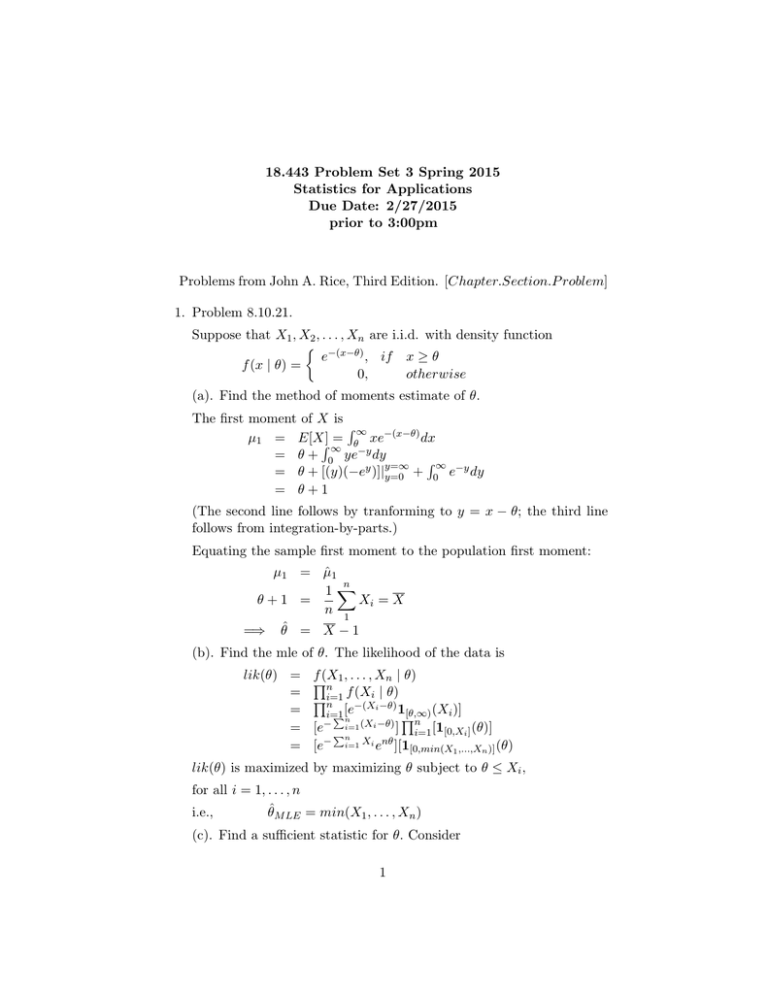
18.443 Problem Set 3 Spring 2015
Statistics for Applications
Due Date: 2/27/2015
prior to 3:00pm
Problems from John A. Rice, Third Edition. [Chapter.Section.P roblem]
1. Problem 8.10.21.
Suppose that X1 , X2 , . . . , Xn are i.i.d. with density function
f (x | θ) =
e−(x−θ) , if
0,
x≥θ
otherwise
(a). Find the method of moments estimate of θ.
The first moment of X is
∞
µ1 = E[X] = θ xe−(x−θ) dx
∞
= θ + 0 ye−y dy
∞ −y
= θ + [(y)(−ey )]|y=∞
y=0 + 0 e dy
= θ+1
(The second line follows by tranforming to y = x − θ; the third line
follows from integration-by-parts.)
Equating the sample first moment to the population first moment:
µ1 = µ̂1
n
1
θ+1 =
Xi = X
n
1
=⇒ θˆ = X − 1
(b). Find the mle of θ. The likelihood of the data is
lik(θ) = ff(X1 , . . . , Xn | θ)
n
=
f (Xi | θ)
fi=1
n
−(Xi −θ) 1
=
[θ,∞) (Xi )]
i=1 [e
f
n
n
−
i=1 (Xi −θ) ]
= [e
i=1 [1[0,Xi ] (θ)]
n
= [e− i=1 Xi enθ ][1[0,min(X1 ,...,Xn )] (θ)
lik(θ) is maximized by maximizing θ subject to θ ≤ Xi ,
for all i = 1, . . . , n
i.e.,
θˆ
M LE = min(X1 , . . . , Xn )
(c). Find a sufficient statistic for θ. Consider
1
T (X1 , . . . , Xn ) = min(X1 , . . . , Xn )
The distribution function of T , FT (t) satisfies
[1 − FT (t)] =
=
=
=
=
P (T > t)
P
1 > t, X2 > t, . . . Xn > t)
f(X
n
P (Xi > t)
fi=1
n
−(t−θ) ]
i=1 [e
−n(t−θ)
[e
]
for values t ≥ θ.
The density of T is simply the derivative:
fT (t | θ) = ne−n(t−θ) , t ≥ θ.
The conditional density of the sample given T = t is
f (X1 , . . . , Xn | θ)
f (X1 , . . . , Xn | T, θ) =
PfnT (t | θ)
[e− i=1 Xi enθ ][1[0,min(X1 ,...,Xn )] (θ)]
=
[e−n(t−θ) ]1[0,t] (θ)
n
Pn
n
= [e− i=1 (Xi −t) ][ 1[t,∞) (Xi )]
i=1
The density function does not depend on θ, so
T = min(X1 , . . . , Xn ) is sufficient for θ.
2. Problem 8.10.45. A Random walk Model for Chromatin
The html in Rproject3.zip ”Rproject3//Rproject3r mdr ayleight heory.html”
details estimation theory for a sample from a Rayleigh distribution.
(a). MLE of θ :
Data consisting of:
R1 , R2 , . . . , Rn
are i.i.d. Rayleigh(θ) random variables. The likelihood function is
f
lik(θ) = f (r1 , . . . , rn | �
θ) = �ni=1 f (ri | θ)
fn � r i
−ri2 �
=
exp
i=1
θ2
2θ2
The log-likelihood function is
£(θ) = log[lik(θ)]
o
= [ n1 log(ri )] − 2nlog(θ) −
2
1
θ2
on
2
1 [ri /2]
The mle solves
d
dθ £(θ)
= 0:
d
= dθ
(£(θ))
o
= −2n( 1θ ) + 2( θ13 ) 1n [ri2 /2]
o
= ( n1 n1 [ri2 /2])1/2
0
=⇒
θ̂M LE
(b). Method of moments estimate:
The first moment of the Rayleigh(θ) distribution is
R∞
µ1 = E[R | θ] = 0 rf (r | θ)dr
R∞ r
r2
= 0
r θ2 exp( −
)dr
2θ2 2
R
∞
r
= θ12 R0 r2
exp( −
)dr
2θ2
∞
−v
1
√ ] (change of variables: v = r 2 )
= θ2 0 v · exp( 2θ2 )[ 2dv
v
R
3
∞
= 2θ12 0
v 2 −1
· exp( 2−θv2 )dv
3
1
2
= √
Γ( 32 )(2θ)√
2θ2
3
=
2θΓ(
) = 2θ × ( 21 )Γ( 21 )
√ 2
= θ × √π2
(using the facts that Γ(n + 1) = nΓ(n) and Γ( 12 ) =
√
π)
The MOM estimate solves:
µ
√1
√π
2
θ×
=⇒ θˆM OM
= µ̂1 =
= R
= R×
1
n
o
Ri
=R
√
√2
π
(c). Approximate Variance of the MLE and method of moments esti­
mate.
The approximate variance of the MLE is V ar(θ̂M LE ) ≈
1
nI(θ)
where
I(θ) =
=
=
=
=
=
2
d
E[− dθ
2 (log(f (x | θ)))]
2
d2
E[− dθ2 [log( θx2 exp(− 2xθ2 ))]]
2
d
E[− dθ
[−2( 1θ ) − ( x2 )(−2)θ−3 ]]
E[−[( θ22 ) + (x2 ))(−3)θ−4 ]]
3θ−4 E[x2 ] − ( θ22 ) = 3θ−4 (2θ2 ) − ( θ22 )
4
θ2
3
So, V ar(θ̂M LE ) ≈
θ2
4n
Variance of the MOM estimate of Rayleigh Distribution Parameter:
The MOM estimate
√
θˆM OM = R × √ 2
π
has variance:
√
V ar(θ̂M OM ) = ( √π2 )2 V ar(R) = ( π2 ) V ar(R)
n
2
V ar(R) = E[R2 ] −
((E[R])
π 2
2
= 2θ − ( 2 θ)
= θ2 (2 − π2 )
So, V ar(θ̂M OM ) = θ2 (2 − π2 )( π2 )( n1 ) = θ2 ( π4 − 1)( n1 ) ≈
This exceeds the approximate V ar(θ̂M LE ) ≈
θ2
n
θ2
n
× 0.2732
× 0.25
See the R script file:
Rproject3 script4 Chromatin solution.r
3. Problem 8.10.51 Double Exponential (Laplace) Distribution
The double exponential distribution is
f (x | θ) = 12 e|x−θ| , −∞ < x < ∞.
For an iid sample of size n = 2m + 1, show that the mle of θ is the
median of the sample.
Let X1 , . . . , Xn denote the sample random variables with outcomes
x1 , . . . , xn . The likelihood function of the data is
fn
fn 1 −|xi −θ|
]
lik(θ) =
i | θ) =
i=1 f (x
i=1 [ 2 e
Pn
1 n − i=1 |xi −θ|
= (2) e
This is maximized by minimizing the sum in the exponent:
o
g(θ) = ni=1 |xi − θ|
Note that g(θ) is a continuous function of θ and its derivative exists
at all points θ that are not equal to any xi
o
d
g / (θ) = dθ
g(θ) =o ni=1 [−1 × 1(xi > θ) + (+1)
on × 1(xi < θ)]
n
= (−1)
×
[
1(x
>
θ)]
+
(+1)
×
i
i=1
i=1 1(xi < θ)]
positive if θ > median(xi )
=
negative if θ < median(xi )
4
It follows that g(θ) is minimized at θ = median(xi ). A graph of g(θ) is
piecewise linear with slope changes at each of the xi values; the slope
at any given θ (not equal to an xj ) is
count(xi < θ) − count(xi > θ).
4. Problem 8.10.58 Gene Frequencies of Haptoglobin Type
Gene frequencies are in equilibrium, the genotypes AA, Aa, and aa oc­
cur with probabilities (1 − θ)2 , 2θ(1 − θ), and θ2 . Plato et al. published
the following data on Haptoglobin Type in a sample of 190 people
Haptoglobin Type
Hp1-1 Hp1-2 Hp2-2
10
68
112
This is precisely the same problem as Example 8.5.1.A of the text
and class notes which corresponds to count data: (X1 , X2 , X3 ) ∼
M ultinomial(n = 3, p = ((1 − θ)2 , 2θ(1 − θ), θ2 ) distribution.
(a). Find the mle of θ
• (X1 , X2 , X3 ) ∼ M ultinomial(n, p = ((1 − θ)2 , 2θ(1 − θ), θ2 ))
• Log Likelihood for θ
£(θ) = log(f (x1 , x2 , x3 | p1 (θ), p2 (θ), p3 (θ)))
= log( x1 !xn!2 !x3 ! p1 (θ)x1 p2 (θ)x2 p3 (θ)x3 )
= x1 log((1 − θ)2 ) + x2 log(2θ(1 − θ))
+x3 log(θ2 ) + (non-θ terms)
= (2x1 + x2 )log(1 − θ) + (2x3 + x2 )log(θ) + (non-θ terms)
• First Differential of log likelihood:
(2x1 + x2 ) (2x3 + x2 )
£/ (θ) = −
+
1 − θ
θ
=⇒ θˆ =
2x3 + x2
2x3 + x2
2(112) + 68
=
=
= 0.76842
2n
2(190)
2x1 + 2x2 + 2x3
(b). Find the asymptotic variance of the mle.
1
E[−£// (θ)]
• Second Differential of log likelihood:
• V ar(θ̂) −→
5
£// (θ) =
d
(2x1 + x2 ) (2x3 + x2 )
[−
+
]
dθ
1−θ
θ
(2x1 + x2 ) (2x3 + x2 )
−
(1 − θ)2
θ2
• Each of the Xi are Binomial(n, pi (θ)) so
E[X1 ] = np1 (θ) = n(1 − θ)2
E[X2 ] = np2 (θ) = n2θ(1 − θ)
E[X3 ] = np3 (θ) = nθ2
2n
• E[−£// (θ)] =
θ(1 − θ)
= −
• σ̂θ̂2 =
θ̂(1 − θ̂)
0.76842(1 − 0.76842)
=
= 0.0004682898 = (.02164)2
2n
2 × 190
Parts (c), (d), and (e): see the R script
Rproject3 script1 multinomial simulation P roblem 8 57.r
6
MIT OpenCourseWare
http://ocw.mit.edu
18.443 Statistics for Applications
Spring 2015
For information about citing these materials or our Terms of Use, visit: http://ocw.mit.edu/terms.