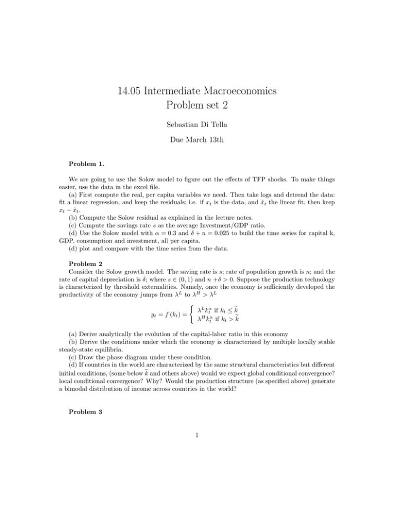
14.05 Intermediate Macroeconomics
Problem set 2
Sebastian Di Tella
Due March 13th
Problem 1.
We are going to use the Solow model to figure out the effects of TFP shocks. To make things
easier, use the data in the excel file.
(a) First compute the real, per capita variables we need. Then take logs and detrend the data:
fit a linear regression, and keep the residuals; i.e. if xt is the data, and x̂t the linear fit, then keep
xt − x̂t .
(b) Compute the Solow residual as explained in the lecture notes.
(c) Compute the savings rate s as the average Investment/GDP ratio.
(d) Use the Solow model with α = 0.3 and δ + n = 0.025 to build the time series for capital k,
GDP, consumption and investment, all per capita.
(d) plot and compare with the time series from the data.
Problem 2
Consider the Solow growth model. The saving rate is s; rate of population growth is n; and the
rate of capital depreciation is δ; where s ∈ (0, 1) and n +δ > 0. Suppose the production technology
is characterized by threshold externalities. Namely, once the economy is sufficiently developed the
productivity of the economy jumps from λL to λH > λL
(
λL ktα if kt ≤ e
k
yt = f (kt ) =
λH ktα if kt > e
k
(a) Derive analytically the evolution of the capital-labor ratio in this economy
(b) Derive the conditions under which the economy is characterized by multiple locally stable
steady-state equilibria.
(c) Draw the phase diagram under these condition.
(d) If countries in the world are characterized by the same structural characteristics but different
initial conditions, (some below e
k and others above) would we expect global conditional convergence?
local conditional convergence? Why? Would the production structure (as specified above) generate
a bimodal distribution of income across countries in the world?
Problem 3
1
Consider an individual who lives for T +1 periods. Let ct denote the consumption in period
t. Denote by yt the exogenous income the agent receives in period t. She has the following
intertemporal utility function
U (c0 , c1 ...cT )
T
X
=
t=0
u0
1
t u (ct )
(1 + δ)
> 0, u00 < 0
where δ is the subjective discount rate. Assume, for simplicity, that the interest rate r = 0 and the
subjective discount rate δ = 0. The agents has wealth a0 to begin with in the first period (t = 0).
(a) Write down the intertemporal budget constraint for this agent.
(b) Write down the agent’s optimization problem to obtain the optimal consumption plan.
Describe how consumption changes with time, does it increase? decreases? [No need to determine
the actual consumption level, just describe how it evolves on time.]
(c) How important is the assumption that r = δ = 0 for your answer in (b)? Can we change
part of the assumption and still get the same result for consumption?
Now assume that the agent’s income is constant in each period, yt = y for every t.
(d) What is the optimal consumption level in each period of life now? How much does the
individual save in period t = 0?
(e) Now suppose that the government announces in t = 0 that will tax individuals. The government implements a tax on income in each period of life such that the agent receives (1 − τ )y each
period, where τ = 1/(1 + T ). How much does the tax reduces the agent’s per-period income? How
much does optimal consumption falls at t = 0?
(f) Now assume that instead of a constant tax rate on each period, the government sets a tax
rate τ = 1 in t = T and 0 in all the earlier periods. How much does the tax reduces the agent’s
per-period income? How much does optimal consumption falls at t = 0?
(g) Compare your answers in parts (e) and (f). Explain the intuition.
2
MIT OpenCourseWare
http://ocw.mit.edu
14.05 Intermediate Macroeconomics
Spring 2013
For information about citing these materials or our Terms of Use, visit: http://ocw.mit.edu/terms.