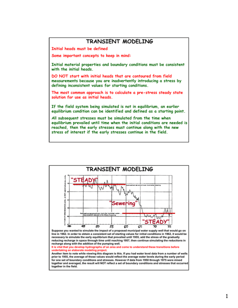
TRANSIENT MODELING
Initial heads must be defined
Some important concepts to keep in mind:
Initial material properties and boundary conditions must be consistent
with the initial heads.
DO NOT start with initial heads that are contoured from field
measurements because you are inadvertently introducing a stress by
defining inconsistent values for starting conditions.
The most common approach is to calculate a pre-stress steady state
solution for use as initial heads.
If the field system being simulated is not in equilibrium
equilibrium, an earlier
equilibrium condition can be identified and defined as a starting point.
All subsequent stresses must be simulated from the time when
equilibrium prevailed until time when the initial conditions are needed is
reached, then the early stresses must continue along with the new
stress of interest if the early stresses continue in the field.
TRANSIENT MODELING
“STEADY”
“Sewering”
“STEADY”
Suppose you wanted to simulate the impact of a proposed municipal water supply well that would go on
g values for initial conditions in 1962,, it would be
line in 1962. In order to obtain a consistent set of starting
necessary to simulate the early equilibrium that prevailed until 1955, add the stress of the gradually
reducing recharge in space through time until reaching 1957, then continue simulating the reductions in
recharge along with the addition of the pumping well.
It is vital that you develop hydrographs of an area and come to understand these transitions before
undertaking an elaborate modeling project.
Another item to note while viewing this diagram is this. If you had water level data from a number of wells
prior to 1955, the average of those values would reflect the average water levels during the early period
for one set of boundary conditions and stresses. However if data from 1950 through 1975 were mixed
together and averaged, the result will NOT reflect a set of boundary conditions and stresses that occurred
together in the field.
1
What can we do if we cannot use a steady state initial condition because our
problem is dependent on a short term response during a particular time of
year? In this case there may be a quasi-cyclic equilibrium in the area, that is a
general repetition of conditions that occur year after year and we may attempt to
represent that situation, then start our stress at the appropriate point in the
cycle. Draw diagrams of the variations and the timing of your stress and
coordinate this with a diagram of model stress periods and time steps to help
yourself get everything timed correctly in your model.
model
What if we do not have sufficient data to establish an acceptable steady
initial condition to commence our cyclic equilibrium? In this case, we may be able
to start with a rather arbitrary initial condition but simulate the cycle long
enough such that we simulate the same values at the same times in subsequent
cycles.
It may
y be that there is enough
g information in your
y
transient data to estimate
initial conditions. This can be judged by evaluating the sensitivity of initial
conditions to the available data and the correlation of parameters defining those
conditions to other parameters that are estimated.
Finally, it is useful to note that the further in time the simulation is from
the initial conditions the less influence those initial conditions have on the
simulated values.
TIME STEPS
time steps are the temporal equivalent of grid cells, they should be small
when stresses change and increase in length to a constant, convenient size
until the stresses change
STRESS PERIODS
stress periods are groups of time steps during which the stresses do not
change
2
Create a transient flow model from the steady state model
TRANSIENT MODELING REQUIRES:
TIME DISCRETIZATION
INITIAL CONDITIONS
STORAGE PARAMETERS
ONE or more S
STRESSES
RESSES
Create a folder for the transient model
Copy in the steady state prediction modflow files
Perhaps rename to indicate they are transient
quick option for renaming in a command window e.g.
copy ep* eptr*
My Transient Files for the Class Example
can be downloaded form the class web page
Consider each file in the name & bat files, edit the name
if you changed it, and determine if it needs changes in
order to conduct a transient simulation
1
2
3
4
5
6
7
8
9
10
3
Transient Parameters
SY = 0.25 in the sand
1.1x that in the more permeable lens
SY = 1.0 in the reservoirs (4 x Sysand but cell 50% sand)
2.5 1.1 1.1 1.0 1.0 1.0 1.0 1.0 1.0 2.5
Do not use a multiplier for reservoirs if you are going to
adjust SY for calibration
Ss = 1x10-6 in both layers
Make these changes in lpf mlt & pval files
Transient Stresses (4 stress periods)
1) simulation starts with a steady state no pumping condition
2) pumping of 3cm3/sec for 5 minutes
3) pumping continues & recharge decreases to 50% for 5 minutes
4) original recharge returns with continued pumping
How long does it take to reach a steady state after that?
Well in layer 1 row 2 column 5
Make changes in dis (see next slide)
oc wel rch mlt riv files
I saved all head and budget information for illustrative purposes
Note the use of instances for the rch variation
Use ob files to print predictions at end of stress periods 2, 3, & 4
4
TRANSIENT MODELING REQUIRES
TIME DISCRETIZATION
dis – increase to 4 periods, defined at the end of the file
At first try 5 steps with a 1.1 multiplier
explore mass balance and storage rates
then adjust #steps and multiplier later
Guess at possible time required to reach SS adjust as
needed after seeing results
1
1
1 SS
300
5 1.1 TR
300
5 1.1 TR
3000 30
1 TR
oc – print the budget for every step so we can explore
for this small model (see oc file in zip file)
RUN MODFLOW
Check lst file
Make sure mass balances are OK at all time steps
Make sure that the cell with the well did not go dry
Check that the heads are reasonable
VERY IMPORTANT TO MAKE SURE THE MODEL MAKES
SENSE AND DOES WHAT YOU EXPECTED:
Using GWChart
View Water Budgets (check modflow,
modflow look at rates)
View Hydrograph for the well cell
Do the graphs make sense?
5