CWP-696
Tensor-guided interpolation on non-planar surfaces
Dave Hale
Center for Wave Phenomena, Colorado School of Mines, Golden CO 80401, USA
a)
b)
c)
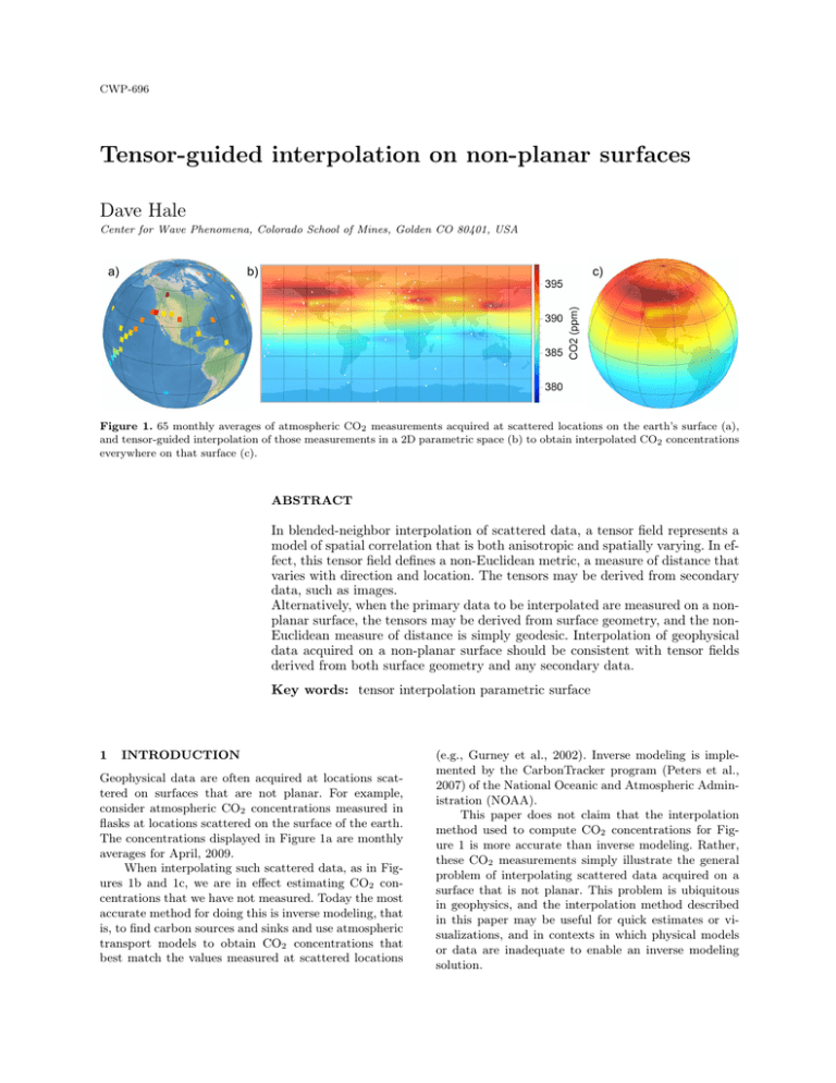
Figure 1. 65 monthly averages of atmospheric CO2 measurements acquired at scattered locations on the earth’s surface (a),
and tensor-guided interpolation of those measurements in a 2D parametric space (b) to obtain interpolated CO2 concentrations
everywhere on that surface (c).
ABSTRACT
In blended-neighbor interpolation of scattered data, a tensor field represents a
model of spatial correlation that is both anisotropic and spatially varying. In effect, this tensor field defines a non-Euclidean metric, a measure of distance that
varies with direction and location. The tensors may be derived from secondary
data, such as images.
Alternatively, when the primary data to be interpolated are measured on a nonplanar surface, the tensors may be derived from surface geometry, and the nonEuclidean measure of distance is simply geodesic. Interpolation of geophysical
data acquired on a non-planar surface should be consistent with tensor fields
derived from both surface geometry and any secondary data.
Key words: tensor interpolation parametric surface
1
INTRODUCTION
Geophysical data are often acquired at locations scattered on surfaces that are not planar. For example,
consider atmospheric CO2 concentrations measured in
flasks at locations scattered on the surface of the earth.
The concentrations displayed in Figure 1a are monthly
averages for April, 2009.
When interpolating such scattered data, as in Figures 1b and 1c, we are in e↵ect estimating CO2 concentrations that we have not measured. Today the most
accurate method for doing this is inverse modeling, that
is, to find carbon sources and sinks and use atmospheric
transport models to obtain CO2 concentrations that
best match the values measured at scattered locations
(e.g., Gurney et al., 2002). Inverse modeling is implemented by the CarbonTracker program (Peters et al.,
2007) of the National Oceanic and Atmospheric Administration (NOAA).
This paper does not claim that the interpolation
method used to compute CO2 concentrations for Figure 1 is more accurate than inverse modeling. Rather,
these CO2 measurements simply illustrate the general
problem of interpolating scattered data acquired on a
surface that is not planar. This problem is ubiquitous
in geophysics, and the interpolation method described
in this paper may be useful for quick estimates or visualizations, and in contexts in which physical models
or data are inadequate to enable an inverse modeling
solution.
250
D. Hale
In the context of exploration geophysics, consider
the interpolation of subsurface properties measured in
boreholes at locations scattered within a geologic layer
bounded by surfaces that are not planar. To simplify
interpolation, we may attempt to flatten the layer and
the bounding surfaces so that they are planar. However,
such flattening may distort distances and, hence, spatial
correlations within the layer (Lee, 2001). Flattening is
unnecessary if we account directly for surface geometry
in the method used to interpolate scattered data.
The interpolation method described in this paper is
a simple extension of the image-guided blended neighbor interpolation method described by Hale (2009). This
method interpolates scattered data using a tensor field
derived from secondary information, such as a seismic
image. In other words, image-guided interpolation is actually tensor-guided, and the tensors that guide interpolation can be derived from many sources, not only
images.
This paper shows that the tensor-guided blended
neighbor method is easily extended to interpolation on
non-planar surfaces defined by a parametric mapping,
because surface geometry simply alters the tensor field
already employed by the method. Using the earth’s surface as a familiar example, I demonstrate this method
for honoring both surface geometry and secondary models for spatial correlation in the interpolation of data
acquired at locations scattered on that surface.
In all of these methods the interpolation of spatially scattered data depends, either explicitly or implicitly, on a model for spatial correlation. In particular, correlation is often assumed to decrease with distance; measurements for any two nearby points tend to
be more similar than those for two distant points. This
dependence on a spatial correlation model is most explicit in statistical methods such as kriging that require
the specification of covariance or variogram functions.
These functions may be anisotropic, but are assumed to
be stationary or at least slowly varying within neighborhoods of known samples. Geostatistical methods such as
kriging are difficult to extend to contexts in which this
stationarity assumption is invalid.
The interpolation method described in this paper
depends explicitly on a model of spatial correlation that
in practice is often highly anisotropic and spatially varying. This model is represented by a tensor field, and the
interpolation is thereby tensor-guided.
The blended neighbor method (Hale, 2009) for
interpolation was developed specifically to facilitate
tensor-guided interpolation. This process consists of two
steps:
Step 1: solve the eikonal equation
rt(x) • D(x) • rt(x) = 1,
t(xk ) = 0,
x2
/ X;
xk 2 X
(4)
for
2
TENSOR-GUIDED INTERPOLATION
Using the notation of Hale (2009), let us assume that
spatially scattered data to be interpolated are a set
F = {f1 , f2 , . . . , fK }
(1)
of K known sample values fk 2 R that correspond to a
set
X = {x1 , x2 , . . . , xK }
(2)
of K known sample points xk 2 Rn . Together these two
sets comprise a set
K = {(f1 , x1 ), (f2 , x2 ), . . . , (fK , xK )}
(3)
of K known samples. These samples may be scattered
such that the n-dimensional sample points in the set
X may have no regular geometric structure. The classic
interpolation problem is to use the known samples in
K to construct a function q(x) : Rn ! R, such that
q(xk ) = fk .
As stated, this problem has no unique solution;
there exist an infinite number of functions q(x) that
satisfy the interpolation conditions q(xk ) = fk . Additional criteria may include measures of smoothness, robustness, and computational efficiency. Because tradeo↵s exist among such criteria, a variety of methods for
interpolating scattered data are commonly used today.
t(x): the minimal time from x to the nearest
known sample point xk , and
p(x): the value fk corresponding to the sample
point xk nearest to the point x.
Step 2: solve the blending equation
q(x)
1
r • t2 (x)D(x) • rq(x) = p(x),
2
(5)
for the blended neighbor interpolant q(x).
The tensor field in this method is denoted by D(x).
At each location x 2 Rn , the tensor D is a symmetric
positive-definite n ⇥ n matrix. The tensor field D(x)
provides a metric, a measure of distance that need not
be Euclidean. Indeed, times t(x) in equation 4 are actually non-Euclidean distances computed for the metric
D(x).
We can get an intuitive sense of the metric D(x)
by considering the special case where D is constant. In
this case, the time (non-Euclidean distance) t(x) from
any known sample point xk to an arbitrary point x can
be computed analytically:
p
t = (x xk ) • D 1 • (x xk ),
(6)
or in matrix-vector notation
p
t = (x xk )T D
1 (x
xk ).
(7)
One can easily verify by substitution that this expres-
Tensor-guided interpolation on non-planar surfaces
251
x2
p
e2
b
p
a
a
e1
contour of
constant time
b
x1
Figure 2. For a metric D(x), contours of constant time (nonEuclidean distance) within any infinitesimal neighborhood
of a point x are elliptical. At each location x, the ellipse
is elongated in the direction in which spatial correlation is
highest.
sion is a solution to the eikonal equation 4, here expressed in matrix-vector notation:
rtT Drt = 1,
(8)
with boundary condition t(xk ) = 0.
For the general case where D(x) is spatially varying, we must compute the solution t(x) of the eikonal
equation 4 numerically. However, even in this case we
may consider an infinitesimally small neighborhood of
any location x, in which D(x) is essentially constant,
and the infinitesimal time dt from x to x + dx is
p
dt = dxT D 1 dx.
(9)
Squaring both sides,
(dt)2 = dxT D
1
dx.
(10)
This last expression is quadratic in dx. Because metric
tensors D (and D 1 ) must be symmetric and positivedefinite, we are assured that (dt)2 0, and a contour of
constant dt is an n-dimensional ellipsoid, as illustrated
for n = 2 in Figure 2.
In 2D each symmetric positive-definite tensor

d11 d12
D=
(11)
d12 d22
is comprised of three unique elements d11 , d12 and d22 .
These three elements are related to the parameters for
the ellipse in Figure 2 by the eigen-decomposition
D=
a aa
T
+
b bb
T
a = cos e1 + sin e2
b=
Figure 3. Ellipses for a tensor field D(x) derived from a
horizontal slice of a 3D seismic image.
sin e1 + cos e2
(12)
where a and b are orthonormal eigenvectors and a and
b their corresponding real and positive eigenvalues, or-
dered such that a
b . Equivalently,

2
+ b sin2
( a
a cos
b ) cos sin
D=
2
( a
+ b cos2
a sin
b ) cos sin
.
(13)
Equations 12 and 13 provide intuitive ways to specify a tensor field D(x) that represents an anisotropic
and spatially varying model of correlation. Where correlation is high, we set both a and b to have large
values. Where correlation is anisotropic, we set a to
be larger than b and we choose the angle to be the
direction in which correlation is highest. All three of the
parameters a , b and may vary with location x.
As an example, Figure 3 shows an example of tensor
ellipses that represent the spatial correlation of features
apparent in a 2D horizontal slice of a 3D seismic image. Correlation in this example is both anisotropic and
spatially varying.
3
ON NON-PLANAR SURFACES
Now let us assume that the data to be interpolated
are acquired at locations scattered on a surface defined
parametrically by a mapping x(u) : U 2 R2 ! X 2 R3 .
For example, on the surface of the earth, scattered data
may be acquired at locations u = (u1 , u2 ) specified by
longitude u1 = and latitude u2 = ✓, and each such
location corresponds to a point x = (x1 , x2 , x3 ) in a
Cartesian earth-centered earth-fixed coordinate system.
Because the space X of points on the surface is a
small subset of R3 , we should not think of our scattered
data as a function of x, but rather as a function of u. It
252
D. Hale
is most convenient to interpolate measurements in the
2D parametric space U 2 R2 in which they are sampled.
In other words, in the blended-neighbor method of
tensor-guided interpolation, we would like to first solve
an eikonal equation:
ru tT Du ru t = 1,
The Jacobian J of the mapping x(u) is defined by
2
3 2 @x1 @x1 3
j11 j12
@u1 @u2
6 @x2 @x2 7
J = [j1 j2 ] = 4j21 j22 5 = 4 @u
(15)
@u2 5 .
1
@x3
@x3
j31 j32
@u1
For example, if we choose the QR decomposition, then
F is a right-triangular matrix with elements that can be
found by Gram-Schmidt orthogonalization.
As illustrated in Figure 4, the tangent spaces J and
E are really the same space, spanned by di↵erent basis
vectors. In choosing the orthonormal vectors e1 and e2
(shown in Figure 2), we choose a basis for specifying a
tensor field De via equation 12, rewritten here as
a aa
+
b bb
T
a = cos e1 + sin e2
b=
u1
x(u)
x
e1
Figure 4. Unit vectors u1 and u2 are mapped to Jacobian
vectors j1 and j2 . These Jacobian vectors and the orthonormal basis vectors e1 and e2 lie in the plane tangent to the
surface at point x = x(u).
orthonormal basis vectors e1 and e2 and eigenvectors a
and b now have three components, as they all lie within
a tangent plane in R3 , not R2 . In particular, the 3 ⇥ 2
matrix E = [e1 e2 ] is not the identity matrix. Using
the 2 ⇥ 2 matrix D defined by equation 13, equation 17
becomes
De = EDET
(18)
re tT De re t = 1.
(19)
To make sense of this eikonal equation in the tangent
space E we must understand how to interpret the intrinsic gradient re t, the gradient within the tangent
space.
@u2
The column vectors j1 and j2 of J are a basis for a
locally planar tangent space J. In any useful surface
parameterization, the vectors j1 and j2 are linearly independent; but their lengths may di↵er, and they need
not be orthogonal. In other words, the vectors j1 and j2
illustrated in Figure 4 may not be the easiest basis in
which to specify the metric tensors D.
We can obtain a tangent space E with orthonormal basis vectors e1 and e2 by decomposition of the
Jacobian matrix J = E F:
3 2
3
2
j11 j12
e11 e12 
4j21 j22 5 = 4e21 e22 5 f11 f12 .
(16)
f21 f22
j31 j32
e31 e32
De =
u
e2
In this way we can easily specify a tensor field De
for an eikonal equation
The tangent space
T
j1
u2
(14)
where Du = Du (u) denotes a tensor field and t = t(u)
denotes non-Euclidean distance, both functions of parametric coordinates u. This eikonal equation leads to the
following question.
How should we compute the tensor field Du (u) so
that our interpolation is consistent with both the geometry of the surface and any model of spatial correlation
specified on that surface?
Equations 12 (or 13) provide an intuitive recipe
for computing metric tensors D in a planar coordinate
space spanned by the orthonormal vectors e1 and e2 .
To extend this recipe to a parametric surface, we must
define a similar locally planar space for every point on
the surface.
3.1
j2
sin e1 + cos e2 .
(17)
In using equation 17 we must remember that the
3.2
The gradients
My interpretation of gradients follows that of Bronstein
et al. (2008). In the parametric space U 2 R2 the gradient ru t has two components
"
#
ru t =
@t
@u1
@t
@u2
,
(20)
and in the Cartesian space X 2 R3 the extrinsic gradient
rx t has three components
2 @t 3
@x
6 @t1 7
rx t = 4 @x
5.
2
(21)
@t
@x3
The parametric and extrinsic gradients are simply
related by the chain rule for di↵erentiation,
@t
@x1 @t
@x2 @t
@x3 @t
=
+
+
,
@uj
@uj @x1
@uj @x2
@uj @x3
(22)
for j = 1, 2, so that
ru t = JT rx t = FT ET rx t.
(23)
In any coordinate space, the gradient of a scalar
field t is defined to be the vector rt for which the dot
product rtT v equals the directional derivative
Dv t(x) ⌘ lim
✏!0
t(x + ✏v)
✏
t(x)
,
(24)
Tensor-guided interpolation on non-planar surfaces
for every vector v in the space. If that vector v is confined to the tangent space E, then using
t(x + ✏v) = t(x) + ✏[rx t(x)]T v + O(✏2 ),
(25)
we have
re tT v = rx tT v.
(26)
For this equation to be satisfied for every vector v in
the tangent space E, the intrinsic gradient re t must
be the projection of the extrinsic gradient rx t onto the
tangent plane at location x on the surface.
This observation is the key to finding a relationship
between the intrinsic gradient re t and the parametric
gradient ru t. We have equation 23 relating ru t and
rx t. If we can find a relationship between re t and rx t,
then we can express re t in terms of ru t, and we will
know how to compute Du (in equation 14) in terms of
De .
The intrinsic gradient re t in the tangent space E
can be written as re t = E c for some coefficients in a
vector c that define the projection of rx t onto E. The
coefficients c are the least-squares solution of E c ⇡ rx t:
ET E c = ET rx t
c = ET rx t
(27)
re t = EET rx t.
(28)
so that
Here the matrix D describes correlation within a local
tangent plane.
As a special case, if our model for spatial correlation on the surface is isotropic and constant (perhaps
because we have no secondary information to the contrary), then D = I and
⇣
⌘ 1
Du = FT F
.
(33)
Distances t(u) are then simply geodesic distances computed by solution of
⇣
⌘ 1
ru tT FT F
ru t = 1.
(34)
In this special case, the tensor field Du (u) accounts for
only the geometry of the surface. Again, because the matrix FT F is symmetric and positive-definite, each tensor
can be represented by an ellipse, as in Figure 2.
4
THE EARTH’S SURFACE
As a simple example, let us consider the parametric
mapping x(u) illustrated in Figure 5. A simple approximation of the earth’s surface is a sphere with constant
radius r, for which an equirectangular parametric mapping is
x1 = r cos cos ✓
Here I have used the fact that the columns e1 and e2 of
E are orthonormal vectors, so that ET E = I.
3.3
253
The parametric tensor field
Combining equations 23 and 28, we can express the intrinsic gradient in terms of the parametric gradient:
re t = EF
T
ru t.
(29)
so that the eikonal equation 14 becomes
ru tT F
1
ET De EF
T
ru t = 1.
(30)
Comparing this equation with equation 14 in parametric
coordinates, we find
x2 = r sin cos ✓
x3 = r sin ✓.
(35)
The parameters are longitude u1 ⌘ and latitude u2 ⌘
✓. For this example, the orthonormal basis vectors e1
and e2 represent easting and northing, respectively, and
the matrix F is

r cos ✓ 0
F=
.
(36)
0
r
Then, assuming that spatial correlation is isotropic and
constant on the earth’s surface (so that D = I),
 1
0
Du = r2 cos2 ✓ 1 .
(37)
0
r2
(32)
Because the matrix Du is diagonal, its e↵ect is to simply
scale the coordinate axes in the parametric space U so
that equation 34 becomes
✓ ◆2
✓ ◆2
1
@t
1 @t
+
= 1,
(38)
r2 cos2 ✓ @
r2 @✓
Du is the tensor field needed to specify the eikonal equation 14 in parametric coordinates. It is the answer to
the question asked above. The matrices F 1 and F T
account for surface geometry, and the 2 ⇥ 2 matrix D
sandwiched between them represents a model of spatial correlation that may be anisotropic and may vary
with location on the surface. Note that this matrix D
is exactly the same as that in equation 13, used to represent correlation for 2D interpolation within a plane.
which is simply the eikonal equation in spherical coordinates, omitting any gradient with respect to radius r,
because r is constant on the surface. Times t( , ✓) computed by solving this equation are geodesic great-circle
distances.
The advantage of the more general eikonal equation 14, with tensor field Du defined by equation 32, is
that we can specify an additional tensor field D representing a model for correlation that varies with location
on the surface of the Earth.
Du = F
1
ET De EF
T
(31)
or, using equation 18,
Du = F
1
DF
T
.
254
D. Hale
Latitude (degrees)
u2 90
0
-90
-180
-90
90
0
Longitude (degrees) u1
180
x3
x1
x2
Figure 5. Parametric (equirectangular) mapping of the
earth’s surface.
4.1
Atmospheric CO2 concentrations
As an example of data recorded on the earth’s surface,
Figure 6 shows monthly averages for April, 2009, of atmospheric CO2 concentrations, measured in flasks at
65 locations scattered around the globe. These data
are made publicly available (ftp://ftp.cmdl.noaa.gov)
by the National Oceanic and Atmospheric Administration (NOAA). CO2 concentrations are expressed as mole
fractions, in parts per million.
To use blended neighbor interpolation as defined by
equations 4 and 5 in the parametric longitude-latitude
space U , we must provide a tensor field Du (u). If we
simply assume that spatial correlation is isotropic and
constant on the earth’s surface, then the tensors are
given by equation 37. Of course, this simple assumption
is unnecessary, because equation 32 can include any tensor field D(u) defined within local tangent planes on the
earth’s surface. What secondary information can help us
define this tensor field D(u)?
Variation with latitude of solar radiation suggests
that CO2 concentrations are likely to vary more in the
Figure 6. Averages of atmospheric CO2 concentrations measured at 65 scattered locations on the earth’s surface in April,
2009.
north-south direction than in the east-west direction.
Such anistropy in spatial correlation can be seen in satellite images of CO2 concentrations in the middle troposphere, provided by the Atmospheric Infrared Sounder
(AIRS) mission of the National Aeronautics and Space
Administration (NASA). We might use these images
to compute anisotropic and spatially-varying tensors D
like those computed from the seismic image shown in
Figure 3. Alternatively, we might use atmospheric transport models to derive these tensors. Unlike methods that
assume stationarity, the blended neighbor interpolation
method can be used for arbitrary tensor fields.
For this example, however, I chose a simpler stationary model of spatial correlation; everywhere on the
earth’s surface, I use the tensor

1 0
D=
.
(39)
1
0 16
The aspect ratio for the corresponding tensor ellipse is
4:1, which implies a correlation distance that is four
times higher in the east-west direction than in the northsouth direction.
In developing this simple model, I computed variograms for the 65 CO2 measurements displayed in Figure 6. Figure 7 shows two such variograms. Each was
computed for geodesic (great-circle) distances in bins
with widths of 10 degrees. The value for each bin is the
rms di↵erence of values for pairs of CO2 measurements
that are separated by the distances for that bin in the
east-west and north-south directions.
Figure 7a shows that di↵erences in CO2 values tend
to be smaller for measurements at stations that are
nearby, and that these di↵erences increase more rapidly
in the north-south direction than in the east-west direction. The ellipse superimposed on this variogram has an
aspect ratio of 4:1, and is roughly a contour of constant
deviation or correlation.
Figure 7b displays a variogram computed in the
same way, after a random permutation of only the CO2
values, not the station locations. No increase (or decrease) in deviation with distance is apparent in this
variogram. Deviations for small distances tend toward
the middle of the range of deviations shown, and tend to
vary less than those for larger distances, simply because
Tensor-guided interpolation on non-planar surfaces
a)
255
a)
b)
b)
Figure 8. Two tensor fields defined for the surface of the
earth. One tensor field (a) is isotropic on the earth spheroid
The other (b) is anisotropic on the earth spheroid, and implies less correlation with distance in the north-south direction than in the east-west direction.
a)
b)
Figure 7. A variogram (a) computed for atmospheric CO2
concentrations measured at 65 scattered locations on the
earth’s surface and (b) for a random permutation of those
same measurements. The ellipse has an aspect ratio of 4:1.
the bins for smaller distances contain more values from
which rms di↵erences are computed. Deviations for bins
at larger distances are both lower and higher and are
less consistent because fewer values contribute to each
bin. This variogram of permuted values implies that the
spatial correlation apparent in Figure 7a is significant.
Figure 8 displays two tensor fields, which correspond to spatial correlation models that are isotropic
(Figure 8a) and anisotropic (Figure 8b) on the surface
of the earth. Note that both tensor fields are anisotropic
and spatially varying in the parametric space of longitude and latitude. However, on the curved surface of the
earth, the tensors displayed in Figure 8a would appear
circular and identical, while those in Figure 8b would
appear elliptical and identical.
Figure 9 displays the corresponding tensor-guided
Figure 9. Tensor-guided interpolations of CO2 concentrations for the (a) isotropic and (b) anisotropic tensor fields
displayed in Figure 8.
blended neighbor interpolations. The interpolation in
Figure 9b is the same as that displayed in Figures 1b
and 1c. As expected, contours of constant CO2 concentration in Figure 9a are more circular, more isotropic,
than those in Figure 9b. The increase in east-west correlation of CO2 concentrations apparent in Figure 9b is
consistent with the anisotropic tensor field in Figure 8b
and the variogram in Figure 7a.
256
5
D. Hale
CONCLUSION
The example in the previous section demonstrates that
the blended neighbor interpolation method can easily
account for an anisotropic model of spatial correlation
on the earth’s surface. However, geostatistical methods
for interpolation, such as kriging, can do this as well for
special surface geometries, such as a sphere.
A distinguishing feature of the blended neighbor
method is its ability to honor non-stationary models
of spatial correlation. These may reflect more general
(non-spherical) surface geometries, such as seismic horizons, as well as spatial correlation apparent in secondary
data, such as seismic or satellite images. More general
and non-stationary models violate fundamental assumptions made by most geostatistical interpolation methods. Such models are therefore seldom used today, but
are easily handled by blended neighbor interpolation.
REFERENCES
Bronstein, A., M. Bronstein, and R. Kimmel, 2008,
Numerical geometry of non-rigid shapes, 1st ed.:
Springer.
Gurney, K., R. M. Law, A. S. Denning, P. J. Rayner,
D. Baker, P. Bousquet, L. Bruhwiler, Y.-H. Chen, P.
Ciais, S. Fan, I. Y. Fung, M. Gloor, M. Heimann,
K. Higuchi, J. John, T. Maki, S. Maksyutov, K.
Masarie, P. Peylin, M. Prather, B. C. Pak, J. Randerson, J. Sarmiento, S. Taguchi, T. Takahashi, and
C.-W. Yuen, 2002, Towards robust regional estimates
of CO2 sources and sinks using atmospheric transport
models: Nature, 415, 626–630.
Hale, D., 2009, Image-guided blended neighbor interpolation of scattered data: 79th Annual International
Meeting, SEG, Expanded Abstracts, 1127–1131.
Lee, R., 2001, Pitfalls in seismic data flattening: The
Leading Edge, 20, 160–164.
Peters, W., A. Jacobson, C. Sweeney, A. Andrews,
T. Conway, K. Masarie, J. Miller, L. Bruhwiler, G.
Pet́ron, A. Hirsch, D. Worthy, G. van der Werf, J.
Randerson, P. Wennberg, M. Krol, and P. Tans, 2007,
An atmospheric perspective on North American carbon dioxide exchange: CarbonTracker: Proceedings of
the National Academy of Sciences, 104, 18925–18930.