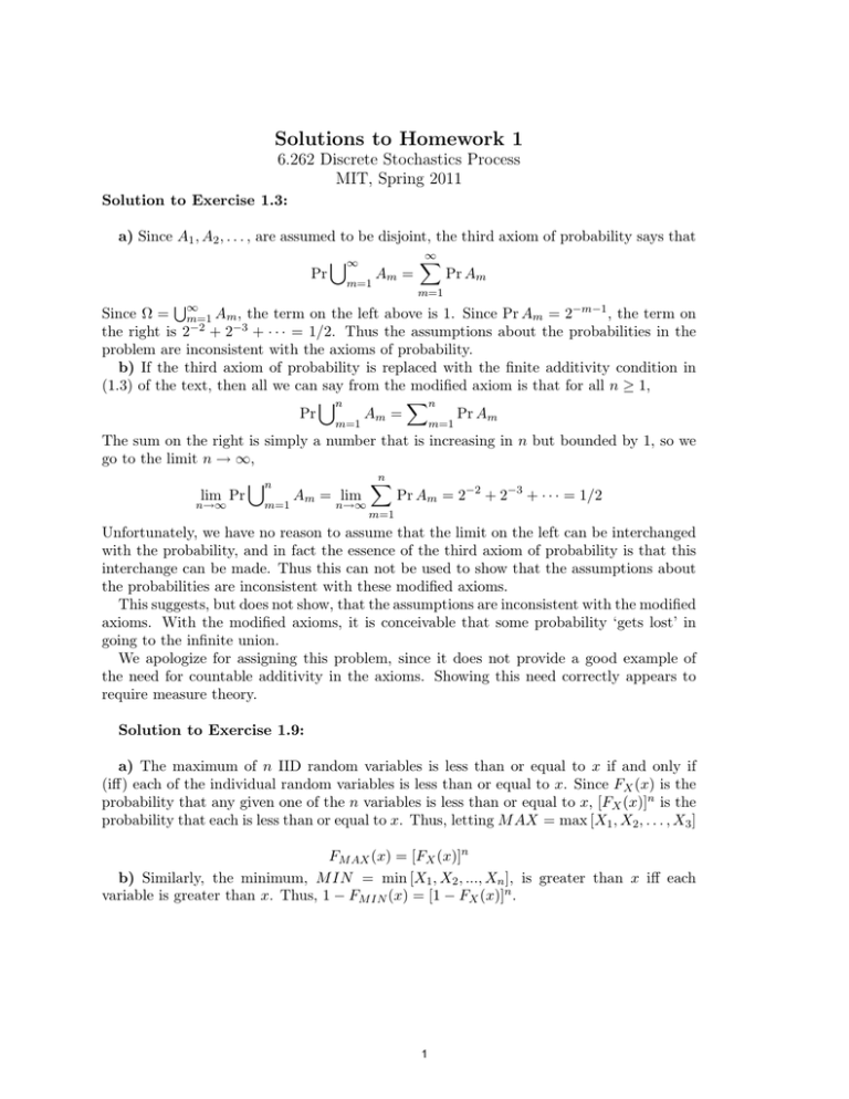
Solutions to Homework 1
6.262 Discrete Stochastics Process
MIT, Spring 2011
Solution to Exercise 1.3:
a) Since A1 , A2 , . . . , are assumed to be disjoint, the third axiom of probability says that
∞
�
∞
Am =
Pr
Pr Am
m=1
m=1
∞
Since Ω = m=1 Am , the term on the left above is 1. Since Pr Am = 2−m−1 , the term on
the right is 2−2 + 2−3 + · · · = 1/2. Thus the assumptions about the probabilities in the
problem are inconsistent with the axioms of probability.
b) If the third axiom of probability is replaced with the finite additivity condition in
(1.3) of the text, then all we can say from the modified axiom is that for all n ≥ 1,
n
�n
Pr
Am =
Pr Am
m=1
m=1
The sum on the right is simply a number that is increasing in n but bounded by 1, so we
go to the limit n → ∞,
n
�
n
lim Pr
Am = lim
Pr Am = 2−2 + 2−3 + · · · = 1/2
n→∞
m=1
n→∞
m=1
Unfortunately, we have no reason to assume that the limit on the left can be interchanged
with the probability, and in fact the essence of the third axiom of probability is that this
interchange can be made. Thus this can not be used to show that the assumptions about
the probabilities are inconsistent with these modified axioms.
This suggests, but does not show, that the assumptions are inconsistent with the modified
axioms. With the modified axioms, it is conceivable that some probability ‘gets lost’ in
going to the infinite union.
We apologize for assigning this problem, since it does not provide a good example of
the need for countable additivity in the axioms. Showing this need correctly appears to
require measure theory.
Solution to Exercise 1.9:
a) The maximum of n IID random variables is less than or equal to x if and only if
(iff) each of the individual random variables is less than or equal to x. Since FX (x) is the
probability that any given one of the n variables is less than or equal to x, [FX (x)]n is the
probability that each is less than or equal to x. Thus, letting M AX = max [X1 , X2 , . . . , X3 ]
FM AX (x) = [FX (x)]n
b) Similarly, the minimum, M IN = min [X1 , X2 , ..., Xn ], is greater than x iff each
variable is greater than x. Thus, 1 − FM IN (x) = [1 − FX (x)]n .
1
c) Let R = M AX − M IN . (See figure)
We start by looking at the joint probability of M AX and M IN by the same technique
used in a) and b). In particular, M AX ≤ x and M IN > y iff y < Xi ≤ x for 1 ≤ i ≤ n.
Thus, Pr(M AX ≤ x, M IN > y) = [FX (x) − FY (y)]n . From the figure, we see that
�
Pr(R ≤ r) =
∂ Pr(M AX ≤ x, M IN > y) ��
dx
�
∂x
y=x−r
�
Assuming that X has a density, this simplifies to nfx (x)[FX (x) − FX (x − r)]n−1 dx
Solution to Exercise 1.13:
a) Since X1 and X2 are identically distributed, Pr(X1 < X2 ) = Pr(X2 < X1 ). Since
Pr(X1 = X2 ) = 0, Pr(X1 < X2 ) = 1/2.
b) Again, using the symmetry between X1 , X2 , and . . . Xn :
Pr(X1 < Xn , X2 < Xn , · · · , Xn−1 < Xn ) = 1/n
.
c) Let’s define In = 1 iff Xn is a record-to-date. Then the expected number of recordto-date that occur over the first m trials is:
2
E[
m
�
In ] =
n=1
=
=
m
�
n=1
m
�
n=1
m
�
n=1
E[In ]
Pr(In = 1)
1
n
The expected number is infinite as m → ∞.
Solution to Exercise 1.20:
a) Suppose Z = (X + Y )mod2 . That is Z = 0 if X = Y and Z = 1 if X =
� Y . Then,
if X and Y are independent, there are 4 joint sample points, (X = 0, Y = 0, Z = 0),
(X = 0, Y = 1, Z = 1), (X = 1, Y = 0, Z = 1) and (X = 1, Y = 1, Z = 0) each of which
have probability 1/4. All other combinations have probability 0. Each pair of random
variable is independent, but the set of three is not.
b) For the example above, the product XY Z is zero with probability 1, and thus
E[XY Z] = 0. On the other hand E [X]E[Y ]E[Z] = (1/2)3 . Thus pairwise independence is
not sufficient for joint independence of all the variables.
Solution to Exercise 1.26:
The algebraic proof of this is straightforward:
FY (y) = Pr(Y ≤ y) = Pr(FX (X) ≤ y)
Note that the set of x satisfying FX (x) ≤ y, i.e., {x : FX (x) ≤ y} is the same as the set
of x for which x ≤ FX−1 (y). (see figure). Thus
(1)
Pr(FX (X) ≤ y) = Pr(X ≤ FX−1 (y)) = FX (FX−1 (y)) = y
If FX (x) is not strictly increasing in x, we define FX−1 (y) as the largest x for which
FX (x) ≤ y so that equation 1 is still satisfied. Since FY (y) = y, the density of Y is given
by
�
1 0≤y≤1
fY (y ) =
0 else
To see what is happening more clearly, consider Pr(y ≤ Y ≤ y + δ) (see figure). The
event y ≤ Y ≤ y + δ is the same as the event FX−1 (x) < x ≤ FX−1 (x + δ). But from
3
the figure, this event has probability (y + δ) − y = δ, meaning again that Y is uniformly
distributed over (0, 1].
Note that the result does not hold for a discrete random variable. For example, if X is
a Bernouli random variable with PX (1) = p and PX (0) = 1 − p, then
⎧
⎨ 0 x < 0
p 0≤x<1
FX (x) =
⎩
1 1≤x
From this we can see that the random variable Y = FX (x) can only take the values p
and 1 (since X can only take on 0 and 1), so Y couldn’t possibly be uniformly distributed
between 0 and 1.
4
MIT OpenCourseWare
http://ocw.mit.edu
6.262 Discrete Stochastic Processes
Spring 2011
For information about citing these materials or our Terms of Use, visit: http://ocw.mit.edu/terms.