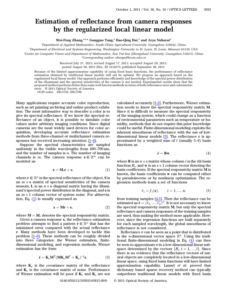
October 1, 2011 / Vol. 36, No. 19 / OPTICS LETTERS
3933
Estimation of reflectance from camera responses
by the regularized local linear model
Wei-Feng Zhang,1,2,* Gongguo Tang,2 Dao-Qing Dai,3 and Arye Nehorai2
1
2
3
Department of Applied Mathematics, South China Agricultural University, Guangzhou 510642, China
Department of Electrical and Systems Engineering, Washington University in St. Louis, St. Louis, Missouri 63130, USA
Center for Computer Vision and Department of Mathematics, Sun Yat-Sen (Zhongshan) University, Guangzhou 510275, China
*Corresponding author: zhangwf@scau.edu.cn
Received July 27, 2011; revised August 17, 2011; accepted August 29, 2011;
posted August 30, 2011 (Doc. ID 151837); published September 30, 2011
Because of the limited approximation capability of using fixed basis functions, the performance of reflectance
estimation obtained by traditional linear models will not be optimal. We propose an approach based on the
regularized local linear model. Our approach performs efficiently and knowledge of the spectral power distribution
of the illuminant and the spectral sensitivities of the camera is not needed. Experimental results show that the
proposed method performs better than some well-known methods in terms of both reflectance error and colorimetric
error. © 2011 Optical Society of America
OCIS codes: 330.1710, 330.1730.
Many applications require accurate color reproduction,
such as art painting archiving and online product exhibition. The most informative way to describe a color is to
give its spectral reflectance. If we know the spectral reflectance of an object, it is possible to simulate color
values under arbitrary imaging conditions. Since digital
cameras are the most widely used devices for color acquisition, developing accurate reflectance estimation
methods from three-channel or multichannel camera responses has received increasing attention [1–6].
Suppose the spectral characteristics are sampled
uniformly in the visible wavelengths from 400–700 nm,
and the number of samples is n. The number of imaging
channels is m. The camera response x ∈ Rm can be
modeled as
x ¼ SLr þ e;
ð1Þ
where r ∈ Rn is the spectral reflectance of the object, S is
an m × n matrix of spectral sensitivities of the camera
sensors, L is an n × n diagonal matrix having the illuminant’s spectral power distribution in the diagonal, and e is
an m × 1 column vector of system noise. For abbreviation, Eq. (1) is usually expressed as
x ¼ Mr þ e;
ð2Þ
where M ¼ SL denotes the spectral responsivity matrix.
Given a camera response x, the reflectance estimation
problem attempts to find a pattern ^r ∈ Rn that has the
minimized error compared with the actual reflectance
r. Many methods have been developed to tackle this
problem [1–6]. These methods can be roughly divided
into three categories: the Wiener estimation, finitedimensional modeling, and regression methods. Wiener
estimation has the form
^r ¼ Kr MT ðMKr MT þ Ke Þ−1 x;
ð3Þ
where Kr is the covariance matrix of the reflectance
and Ke is the covariance matrix of noise. Performance
of Wiener estimation will be poor if Kr and Ke are not
0146-9592/11/193933-03$15.00/0
calculated accurately [1,2]. Furthermore, Wiener estimation needs to know the spectral responsivity matrix M.
Since it is difficult to measure the spectral responsivity
of the imaging system, which could change as a function
of environmental parameters such as temperature or humidity, methods that do not require this prior knowledge
could be useful. Finite-dimensional modeling exploits the
inherent smoothness of reflectance with the use of lowdimensional linear models [3]. The reflectance r is approximated by a weighted sum of l (usually 5–8) basis
functions as
^r ¼ Bw;
ð4Þ
where B is an n × s matrix whose column i is the ith basis
function Bi , and w is an s × 1 column vector denoting the
basis coefficients. If the spectral responsivity matrix M is
known, the basis coefficients w can be computed either
by pseudoinverse or by nonlinear optimization. The regression methods learn a set of functions
^r i ¼ f i ðxÞ;
i ¼ 1; …; n;
ð5Þ
from training samples [4,5]. Then the reflectance can be
estimated as ^r ¼ ð^r 1 ; …; ^r n ÞT . It is not necessary to know
the spectral responsivity matrix M, but only the spectral
reflectance and camera responses of the training samples
are used, thus making the method more applicable. However, since the regression functions are built separately
for each sampled wavelength, the global smoothness of
reflectance is not considered.
Reflectance r can be seen as a point that is distributed
in the n-dimensional vector space Rn . Using the traditional finite-dimensional modeling in Eq. (4) can then
be seen to approximate r in a low-dimensional linear subspace determined by the vectors fBi ; i ¼ 1; …; lg. Since
there is no evidence that the reflectance vectors of natural objects are completely located in a low-dimensional
linear space, using fixed basis functions will have limited
approximation capability. Lansel et al. proved that
dictionary based sparse recovery method can typically
outperform traditional linear models with fixed basis
© 2011 Optical Society of America
3934
OPTICS LETTERS / Vol. 36, No. 19 / October 1, 2011
functions [6]. However, their method is computationally
intensive and needs to know the spectral responsivity
matrix M.
In this Letter, we propose a novel reflectance estimation approach based on the regularized local linear model
(RLLM). The reflectance r for a camera response x is approximated adaptively by the linear combination of k reflectances from the training set that have similar camera
responses to x. The idea is inspired by the regularized
locality preserving method for the preimage problem
in kernel principal component analysis [7]. Our method
is efficient and we do not need to know the spectral
responsivity matrix M.
Local linear model. Although, in a global view, the
reflectance vectors are not located in a low-dimensional
linear subspace, we expect each reflectance and its
neighbors to lie on or close to a locally linear lowdimensional subspace. Since similar reflectances usually
have similar camera responses, we can build the local
linear model as
r¼
Σki¼1 wi ri ;
ð6Þ
where fri ; i ¼ 1; …; kg are reflectances from the training
set that have similar camera responses to x. The reconstruction weight w ¼ ðwi ; …; wk ÞT in Eq. (6) is computed
by regularized linear regression as follows.
Regularized linear regression. For a given camera
response x, let fx1 ; …; xk g be its k nearest neighbors by
Euclidean distance from the training set, and fr1 ; …; rk g
be the corresponding reflectances of fx1 ; …; xk g. By substituting Eq. (6) into Eq. (2), we have the relationship
x ≈ Σki¼1 wi xi :
ð7Þ
Table 1. Summary of Datasets
Dataset
Training set
Testing set
Validation set
Name
Size
Munsell Matte
Agfa IT8.7/2
Paper
100, 300, 600, 900
288
426
Thus we can learn the local linear reconstruction weight
w ¼ ðwi ; …; wk ÞT in Eq. (6) by solving the regularized
linear regression problem
2
k
X
2
arg minw x −
wi xi þλkwk ;
ð8Þ
i¼1
where the regularization parameter λ is used to prevent
overfitting. Let X be an m × k matrix in which column i
is the ith nearest camera responses xi . Then the solution
of Eq. (8) can be given by
w ¼ ðXT X þ λIÞ−1 XT x;
ð9Þ
where I is a k × k identity matrix.
Experimental results. We compare the performance of
our method with five other methods: linear least squares
regression (LLS), finite-dimensional modeling using the
first five or 10 principal component analysis (PCA) basis
vectors, whose basis coefficients are computed by linear
least squares regression, and kernel regression with the
Gaussian kernel and the Dochon spline kernel [4]. Note
that our experiments are under the assumption that the
spectral responsivity matrix M is unknown, so Wiener
estimation and other methods that need to know M
are not compared here.
Table 2. Estimation Errors of Different Methods on the Validation Seta
Error Term
Training Size
100
300
RMSE
600
900
100
300
ΔE 00 ðD65Þ
600
900
100
300
ΔE 00 ðAÞ
600
900
a
Mean
Max
Mean
Max
Mean
Max
Mean
Max
Mean
Max
Mean
Max
Mean
Max
Mean
Max
Mean
Max
Mean
Max
Mean
Max
Mean
Max
LLS
PCA-5
PCA-10
G-Kernel
D-Kernel
RLLM
0.0513
0.0552
0.0511
0.0533
0.0505
0.0513
0.0507
0.0513
1.8683
2.3566
1.8356
1.9508
1.8051
1.8437
1.8108
1.8514
3.3735
3.9730
3.3208
3.5680
3.2760
3.3769
3.2832
3.3515
0.0513
0.0552
0.0511
0.0533
0.0505
0.0513
0.0507
0.0513
1.8694
2.3510
1.8377
1.9522
1.8078
1.8465
1.8134
1.8553
3.3788
3.9574
3.3263
3.5707
3.2809
3.3825
3.2883
3.3587
0.0513
0.0552
0.0511
0.0533
0.0505
0.0513
0.0507
0.0513
1.8682
2.3566
1.8356
1.9508
1.8051
1.8437
1.8108
1.8514
3.3735
3.9730
3.3208
3.5680
3.2760
3.3769
3.2832
3.3515
0.0505
0.0550
0.0489
0.0519
0.0481
0.0498
0.0479
0.0488
1.9194
2.7644
1.6736
1.9601
1.5900
1.8010
1.5678
1.6248
2.9204
3.3906
2.5791
3.0125
2.4743
2.6460
2.4296
2.5211
0.0512
0.0544
0.0501
0.0529
0.0497
0.0513
0.0499
0.0510
2.0592
3.9811
1.9102
2.3052
1.7891
1.8605
1.7851
1.8340
3.4429
4.1571
3.2446
3.6729
3.1428
3.4343
3.1249
3.3743
0.0475
0.0521
0.0457
0.0492
0.0444
0.0454
0.0444
0.0452
1.7004
2.0473
1.5622
1.7912
1.4928
1.5546
1.5122
1.5660
2.5485
3.0835
2.2283
2.4980
2.1220
2.2323
2.1290
2.2062
For each training data size, the results are summarized over 50 trials. In each row the best result is rendered in bold type.
October 1, 2011 / Vol. 36, No. 19 / OPTICS LETTERS
Three datasets of spectral reflectance are used for evaluation and are shown in Table 1. They are all obtained
from [8]. Camera responses are simulated based on the
spectral sensitivity curves of a real three-channel camera
measured by Barnard et al. [9]. The illumination light is assumed to be the Commission Internationale de l’Eclairage
illuminant D65. The spectra of datasets and the sensor
sensitivities are sampled from 400 to 700 nm in 10 nm
increments.
Different-sized training sets are randomly selected
from the 1269 samples of the Munsell dataset. The training set is used to build the regression functions for the
regression methods, compute the PCA basis set for the
finite-dimensional modeling, and compute the k nearest
neighbors for our method. The testing set is used to
select the optimal parameters of the kernel regression
methods and our method. The best parameters are chosen empirically from predefined sets. The idea is to find
parameters that minimize the reflectance error on the
testing set. Finally, the generalization performance of the
six methods is assessed on the validation set.
Table 2 shows the reflectance errors and colorimetric
errors of different methods on the validation set. For
each training data size, the results are summarized over
50 trials. As can be seen, our method provides the lowest
reflectance errors and colorimetric errors in every training set size. Kernel regression methods seem to perform
better than the linear least squares regression method. In
the case of small training set size (100 samples), kernel
regression provides slightly lower reflectance errors than
the linear least squares regression but higher colorimetric errors. However, when increasing the number
of training samples, it is evident that kernel regression
performs much better than linear least squares regression. This verifies that the nonlinear regression methods
are more suitable for large training set sizes. The performance of finite-dimensional modeling with PCA basis
sets is close to that of the linear least squares regression
method. The more the principal components are used,
the closer the performance is. This proves, in a sense,
that the performance of reflectance approximation in
the global space cannot be improved by using a fixed
low-dimensional subspace in it.
3935
The performance of our method depends on the
choices of the regularization parameter λ and the number
of nearest neighbors k. Through evaluation, we find our
method is not sensitive to these two parameters. The results of our method in Table 2 are given by setting k ¼ 20
and λ ¼ 0:0001. For the different-sized randomly selected
training sets, setting k ¼ 20 and λ ¼ 0:0001 can always
give satisfactory results. The results given by k ¼ 20;
30; 40, and 50 are very similar. The camera responses
of the experimental data in Table 2 are simulated with
no noise added. We have also investigated the spectral
estimation accuracy under two different levels of simulated independent Gaussian noise. We find our method
still performs the best.
In summary, our local linear model focuses on the individual reflectance estimation performance rather than
on building a global model that fits all the training samples. It performs adaptively and efficiently, and needs
mainly the low-order matrix inverse operation. Furthermore, our method does not require prior knowledge of
the spectral power distribution of the illuminant and
the spectral sensitivities of the camera.
This work was supported in part by the National
Natural Science Foundation of China (NSFC, grants
60903094, 11171354, and 90920007).
References
1. N. Shimano, K. Terai, and M. Hironaga, J. Opt. Soc. Am. A
24, 3211 (2007).
2. H. L. Shen and J. H. Xin, Opt. Lett. 32, 96 (2007).
3. X. Zhang and H. Xu, J. Opt. Soc. Am. A 25, 371 (2008).
4. V. Heikkinen, T. Jetsu, J. Parkkinen, M. Hauta-Kasari,
T. Jaaskelainen, and S. D. Lee, J. Opt. Soc. Am. A 24, 2673
(2007).
5. W.-F. Zhang and D.-Q. Dai, J. Opt. Soc. Am. A 25, 2286
(2008).
6. S. Lansel, M. Parmar, and B. A. Wandell, Proc. SPIE 7246,
72460D (2009).
7. W.-S. Zheng and J.-H. Lai, in Proceedings of the 18th International Conference on Pattern Recognition (2006), Vol. 2,
pp. 456–459.
8. Spectral database, University of Joensuu Color Group,
http://spectral.joensuu.fi/.
9. K. Barnard, L. Martin, B. Funt, and A. Coath, Color Res.
Appl. 27, 147 (2002).