2
Graphs, Diffusion Maps, and Semi-supervised Learning
2.1
Graphs
Graphs will be one of the main objects of study through these lectures, it is time
to introduce them.
V
A graph G = (V, E) contains a set of nodes V = {v1 , . . . , vn } and edges E ⊆ 2 . An edge (i, j) ∈ E
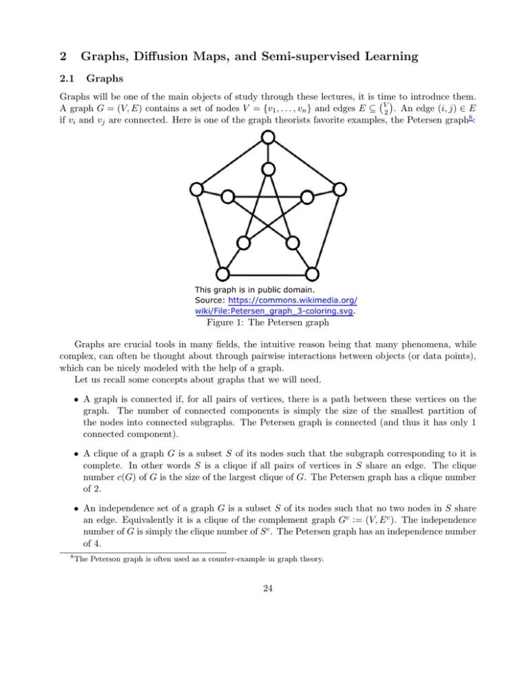
if vi and vj are connected. Here is one of the graph theorists favorite examples, the Petersen graph8 :
This graph is in public domain.
Source: https://commons.wikimedia.org/
wiki/File:Petersen_graph_3-coloring.svg.
Figure 1: The Petersen graph
Graphs are crucial tools in many fields, the intuitive reason being that many phenomena, while
complex, can often be thought about through pairwise interactions between objects (or data points),
which can be nicely modeled with the help of a graph.
Let us recall some concepts about graphs that we will need.
• A graph is connected if, for all pairs of vertices, there is a path between these vertices on the
graph. The number of connected components is simply the size of the smallest partition of
the nodes into connected subgraphs. The Petersen graph is connected (and thus it has only 1
connected component).
• A clique of a graph G is a subset S of its nodes such that the subgraph corresponding to it is
complete. In other words S is a clique if all pairs of vertices in S share an edge. The clique
number c(G) of G is the size of the largest clique of G. The Petersen graph has a clique number
of 2.
• An independence set of a graph G is a subset S of its nodes such that no two nodes in S share
an edge. Equivalently it is a clique of the complement graph Gc := (V, E c ). The independence
number of G is simply the clique number of S c . The Petersen graph has an independence number
of 4.
8
The Peterson graph is often used as a counter-example in graph theory.
24
A particularly useful way to represent a graph is through its adjacency matrix. Given a graph
G = (V, E) on n nodes (|V | = n), we define its adjacency matrix A ∈ Rn×n as the symmetric matrix
with entries
1 if (i, j) ∈ E,
Aij =
0 otherwise.
Sometime, we will consider weighted graphs G = (V, E, W ), where edges may have weights wij ,
we think of the weights as non-negative wij ≥ 0 and symmetric wij = wji .
2.1.1
Cliques and Ramsey numbers
Cliques are important structures in graphs and may have important application-specific applications.
For example, in a social network graph (e.g., where people correspond to vertices and two vertices are
connected if the respective people are friends) cliques have a clear interpretation.
A natural question is whether it is possible to have arbitrarily large graphs without cliques (and
without it’s complement having cliques), Ramsey answer this question in the negative in 1928 [Ram28].
Let us start with some definitions: given a graph G we define r(G) as the size of the largest clique of
independence set, i.e.
r(G) := max {c(G), c (Gc )} .
Given r, let R(r) denote the smallest integer n such that every graph G on n nodes must have r(G) ≥ r.
Ramsey [Ram28] showed that R(r) is finite, for every r.
Remark 2.1 It is easy to show that R(3) ≤ 6, try it!
We will need a simple estimate for what follows (it is a very useful consequence of Stirling’s
approximation, e.g.).
Proposition 2.2 For every k ≤ n positive integers,
n k n ne k
≤
≤
.
r
k
k
We will show a simple lower bound on R(r). But first we introduce a random graph construction,
an Erdős-Renyı́ graph.
Definition 2.3 Given n and p, the random Erdős-Renyı́ graph G(n, p) is a random graph on n vertices
where each possible edge appears, independently, with probability p.
The proof of the lower bound on R(r) is based on the probabilistic method, a beautiful nonconstructive method pioneered by Paul Erdős to establish the existence of certain objects. The core
idea is the simple observation that if a random variable has a certain expectation then there must exist
a draw of it whose value is at least that of the expectation. It is best understood with an example.
Theorem 2.4 For every r ≥ 2,
R(r) ≥ 2
25
r−1
2
.
Proof. Let G be drawn from the G n, 21 distribution, G ∼ G n, 12 . For every set S of r nodes, let
X(S) denote the random variable
1 if S is a clique or independent set,
X(S) =
0 otherwise.
Also, let X denote the random variable
X
X=
V
r
S∈(
X(S).
)
We will proceed by estimating E [X]. Note that, by linearity of expectation,
X
E [X] =
E [X(S)] ,
V
S∈( r )
2
|S | . This means that
(
2 2)
X
n
2
2
n 2
=
=
E [X] =
.
r
|S|
r(r−1)
)
(
r
r
(2)
22
2 2
S ∈(V ) 2
and E [X(S)] = Prob {S is a clique or independent set} =
r
By Proposition 2.2 we have,
E [X] ≤
2
ne r
r
2
r(r−1)
2
=2
n e
r−1
2 2 r
r
.
r−1
That means that if n ≤ 2 2 and r ≥ 3 then E [X] < 1. This means that Prob{X < 1} > 0 and since
X is a non-negative integer we must have Prob{X = 0} = Prob{X < 1} > 0 (another way of saying
that is that if E [X] < 1 then there must be an instance for which X < 1 and since X is a non-negative
r−1
integer, we must have X = 0). This means that there exists a graph with 2 2 nodes that does not
have cliques or independent sets of size r which implies the theorem.
2
Remarkably, this lower bound is not very different from the best known. In fact, the best known
lower and upper bounds known [Spe75, Con09] for R(r) are
√ 2r √ r
− c log r
(1 + o(1))
2 ≤ R(r) ≤ r log log r 4r .
(22)
e
Open Problem 2.1 Recall the definition of R(r) above, the following questions are open:
• What is the value of R(5)?
• What are the asymptotics
of R(s)? In particular, improve on the base of the exponent on either
√
the lower bound ( 2) or the upper bound (4).
26
• Construct a family of graphs G = (V, E) with increasing number of vertices for which there exists
ε > 0 such that9
|V | . (1 + ε)r .
It is known that 43 ≤ R(5) ≤ 49. There is a famous quote in Joel Spencer’s book [Spe94] that
conveys the difficulty of computing Ramsey numbers:
“Erdős asks us to imagine an alien force, vastly more powerful than us, landing on Earth and
demanding the value of R(5) or they will destroy our planet. In that case, he claims, we should
marshal all our computers and all our mathematicians and attempt to find the value. But suppose,
instead, that they ask for R(6). In that case, he believes, we should attempt to destroy the aliens.”
There is an alternative useful way to think about 22, by taking log2 of each bound and rearranging,
we get that
1
min
r(G) ≤ (2 + o(1)) log2 n
+ o(1) log2 n ≤
2
G=(V,E), |V |=n
The current “world record” (see [CZ15, Coh15]) for deterministic construction of families of graphs with
c
small r(G) achieves r(G) . 2(log log |V |) , for some constant c > 0. Note that this is still considerably
larger than polylog|V |. In contrast, it is very easy for randomized constructions to satisfy r(G) ≤
2 log2 n, as made precise by the folloing theorem.
Theorem 2.5 Let G ∼ G n, 12 be and Erdős-Renyı́ graph with edge probability 21 . Then, with high
probability,10
R(G) ≤ 2 log2 (n).
Proof. Given n, we are interested in upper bounding Prob {R(G) ≥ d2 log2 ne}. and we proceed by
union bounding (and making use of Proposition 2.2):
Prob {R(G) ≥ d2 log2 ne} = Prob ∃S⊂V, |S |=d2 log2 ne S is a clique or independent set






[
= Prob
{S is a clique or independent set}


S∈

V
(d2 log2 ne)
X
≤
Prob {S is a clique or independent set}
V
S ∈(d2 log ne)
2
n
2
=
d2 log2 ne
d2 log2 ne 2( 2 )
!d2 log2 ne
n
e
≤ 2
d2 log2 ne−1
d2 log2 ne
2
2
√ !d2 log2 ne
e 2
≤ 2
2 log2 n
. n−Ω(1) .
9
10
By ak . bk we mean that there exists a constant c such that ak ≤ c bk .
We say an event happens with high probability if its probability is ≥ 1 − n−Ω(1) .
27
2
The following is one of the most fascinating conjectures in Graph Theory
Open Problem 2.2 (Erdős-Hajnal Conjecture [EH89]) Prove or disprove the following:
For any finite graph H, there exists a constant δH > 0 such that any graph on n nodes that does
not contain H as a subgraph (is a H-free graph) must have
r(G) & nδH .
√
It is known that r(G) & exp cH log n , for some constant cH > 0 (see [Chu13] for a survey
on this conjecture). Note that this lower bound already shows that H-free graphs need to have
considerably larger r(G). This is an amazing local to global effect, where imposing a constraint on
small groups of vertices are connected (being H-free is a local property) creates extremely large cliques
or independence sets (much larger than polylog(n) as in random Erdős-Renyı́ graphs).
Since we do not know how to deterministically
construct graphs with r(G) ≤ polylogn, one ap
proach could be to take G ∼ G n, 21 and check that indeed it has small clique and independence
number. However, finding the largest clique on a graph is known to be NP-hard (meaning that there
is no polynomial time algorithm to solve it, provided that the widely believed conjecture N P 6= P
holds). That is a worst-case statement and thus it doesn’t necessarily mean that it is difficult to find
the clique number of random graphs. That being said, the next open problem suggests that this is
indeed still difficult.
First let us describe a useful construct. Given
n and ω, let us consider a random graph G that
consists of taking a graph drawn from G n, 21 , picking ω of its nodes (say at random) and adding an
edge between every pair of those ω nodes, thus “planting” a clique of size ω. This will create a clique
of size ω in G. If ω > 2 log2 n this clique is larger than any other clique that was in the graph before
planting. This means that, if ω > 2 log2 n, there is enough information in the graph to find the planted
clique. In fact, one can simply look at all subsets of size 2 log2 n + 1 and check wether it is clique: if
it is a clique then it very likely these vertices belong to the planted clique. However, checking all such
subgraphs takes super-polynomial time ∼ nO(log n) . This motivates the natural question of whether
this can be done in polynomial time.
√
Since the degrees of the nodes of a G n, 12 have expected value n−1
and standard deviation ∼ n,
2
√
if ω > c n (for sufficiently large constant c) then the degrees of the nodes involved in the planted
clique will have larger degrees and it is easy to detect (and find) the planted clique. Remarkably,
there is no known method to work for ω significant smaller than this. There is a quasi-linear
time
pn
√ 11
algorithm [DM13] that finds the largest clique, with high probability, as long as ω ≥ e + o( n).
Open Problem
2.3 (The planted clique problem) Let G be a random graph constructed by tak
ing a G n, 12 and planting a clique of size ω.
1. Is there a polynomial time algorithm that is √
able to find the largest clique of G (with high prob√
ability) for ω n. For example, for ω ≈ lognn .
√
There is an amplification technique that allows one to find the largest clique for ω ≈ c n for arbitrarily small c in
polynomial time, where the exponent in the runtime depends on c. The rough idea is to consider all subsets of a certain
finite size and checking whether the planted clique contains them.
11
28
2. Is there a polynomial time algorithm that is able to distinguish,
with high probability, G from a
√
√
n
1
draw of G n, 2 for ω n. For example, for ω ≈ log n .
3. Is there a quasi-linear
√ time algorithm able to find the largest clique of G (with high probability)
1
for ω ≤ √e − ε
n, for some ε > 0.
This open problem is particularly important. In fact, the hypothesis that finding planted cliques
for small values of ω is behind several cryptographic protocols, and hardness results in average case
complexity (hardness for Sparse PCA being a great example [BR13]).
2.2
Diffusion Maps
Diffusion Maps will allows us to represent (weighted) graphs G = (V, E, W ) in Rd , i.e. associating,
to each node, a point in Rd . As we will see below, oftentimes when we have a set of data points
x1 , . . . , xn ∈ Rp it will be beneficial to first associate to each a graph and then use Diffusion Maps to
represent the points in d-dimensions, rather than using something like Principal Component Analysis.
Before presenting Diffusion Maps, we’ll introduce a few important notions. Given G = (V, E, W )
we consider a random walk (with independent steps) on the vertices of V with transition probabilities:
Prob {X(t + 1) = j|X(t) = i} =
where deg(i) =
P
j
wij
,
deg(i)
wij . Let M be the matrix of these probabilities,
Mij =
wij
.
deg(i)
It is easy to see that Mij ≥ 0 and M 1 = 1 (indeed, M is a transition probability matrix). Defining D
as the diagonal matrix with diagonal entries Dii = deg(i) we have
M = D−1 W.
If we start a random walker at node i (X(0) = 1) then the probability that, at step t, is at node j
is given by
Prob {X(t) = j|X(0) = i} = M t ij .
In other words, the probability cloud of the random walker at point t, given that it started at node i
is given by the row vector
Prob {X(t)|X(0) = i} = eTi M t = M t [i, :].
Remark 2.6 A natural representation of the graph would be to associate each vertex to the probability
cloud above, meaning
i → M t [i, :].
This would place nodes i1 and i2 for which the random walkers starting at i1 and i2 have, after t steps,
very similar distribution of locations. However, this would require d = n. In what follows we will
construct a similar mapping but for considerably smaller d.
29
1
1
1
1
M is not symmetric, but a matrix similar to M, S = D 2 M D− 2 is, indeed S = D− 2 W D− 2 . We
consider the spectral decomposition of S
S = V ΛV T ,
where V = [v1 , . . . , vn ] satisfies V T V = In×n and Λ is diagonal with diagonal elements Λkk = λk (and
we organize them as λ1 ≥ λ2 ≥ · · · ≥ λn ). Note that Svk = λk vk . Also,
1 T
1
1
1
1
1
M = D− 2 SD 2 = D− 2 V ΛV T D 2 = D− 2 V Λ D 2 V
.
1
1
We define Φ = D− 2 V with columns Φ = [ϕ1 , . . . , ϕn ] and Ψ = D 2 V with columns Ψ = [ψ1 , . . . , ψn ].
Then
M = ΦΛΨT ,
and Φ, Ψ form a biorthogonal system in the sense that ΦT Ψ = In×n or, equivalently, ϕTj ψk = δjk .
Note that ϕk and ψk are, respectively right and left eigenvectors of M , indeed, for all 1 ≤ k ≤ n:
M ϕk = λ k ϕk
and ψkT M = λk ψkT .
Also, we can rewrite this decomposition as
M=
n
X
λk ϕk ψkT .
k=1
and it is easy to see that
t
M =
n
X
λtk ϕk ψkT .
(23)
k=1
Let’s revisit the embedding suggested on Remark 2.6. It would correspond to
vi → M t [i, :] =
n
X
λtk ϕk (i)ψkT ,
k=1
it is written in terms of the basis ψk . The Diffusion Map will essentially consist of the representing a
node i by the coefficients of the above map
 t

λ1 ϕ1 (i)
 λt ϕ2 (i) 

 2
(24)
vi → M t [i, :] = 
,
..


.
λtn ϕn (i)
Note that M 1 = 1, meaning that one of the right eigenvectors ϕk is simply a multiple of 1 and so it
does not distinguish the different nodes of the graph. We will show that this indeed corresponds to
the the first eigenvalue.
Proposition 2.7 All eigenvalues λk of M satisfy |λk | ≤ 1.
30
Proof.
Let ϕk be a right eigenvector associated with λk whose largest entry in magnitude is positive
ϕk (imax ). Then,
n
X
λk ϕk (imax ) = M ϕk (imax ) =
Mimax ,j ϕk (j) .
j=1
This means, by triangular inequality that, that
|λk | =
n
X
j=1
n
|Mimax ,j |
X
|ϕk (j)|
≤
|Mimax ,j | = 1.
|ϕk (imax )|
j=1
2
Remark 2.8 It is possible that there are other eigenvalues with magnitude 1 but only if G is disconnected or if G is bipartite. Provided that G is disconnected, a natural way to remove potential
periodicity issues (like the graph being bipartite) is to make the walk lazy, i.e. to add a certain probability of the walker to stay in the current node. This can be conveniently achieved by taking, e.g.,
1
1
M 0 = M + I.
2
2
By the proposition above we can take ϕ1 = 1, meaning that the first coordinate of (24) does not
help differentiate points on the graph. This suggests removing that coordinate:
Definition 2.9 (Diffusion Map) Given a graph G = (V, E, W ) construct M and its decomposition
M = ΦΛΨT as described above. The Diffusion Map is a map φt : V → Rn−1 given by
 t

λ2 ϕ2 (i)
 λt ϕ3 (i) 
 3

φt (vi ) = 
.
..


.
λtn ϕn (i)
This map is still a map to n − 1 dimensions. But note now that each coordinate has a factor of
λtk which, if λk is small will be rather small for moderate values of t. This motivates truncating the
Diffusion Map by taking only the first d coefficients.
Definition 2.10 (Truncated Diffusion Map) Given a graph G = (V, E, W ) and dimension d, construct M and its decomposition M = ΦΛΨT as described above. The Diffusion Map truncated to d
dimensions is a map φt : V → Rd given by


λt2 ϕ2 (i)
 λt ϕ3 (i) 
3


(d)
φt (vi ) = 
.
..


.
λtd+1 ϕd+1 (i)
31
In the following theorem we show that the euclidean distance in the diffusion map coordinates
(called diffusion distance) meaningfully measures distance between the probability clouds after t iterations.
Theorem 2.11 For any pair of nodes vi1 , vi2 we have
kφt (vi1 ) − φt (vi2 )k2 =
n
X
j=1
1
[Prob {X(t) = j|X(0) = i1 } − Prob {X(t) = j|X(0) = i2 }]2 .
deg(j)
Proof.
P
2
1
Note that nj=1 deg(j
) [Prob {X(t) = j|X(0) = i1 } − Prob {X(t) = j |X(0) = i2 }] can be rewritten
as
" n
" n
#2
#2
n
n
n
X
X
X
X
X
1
1
t
t
t
λk ϕk (i1 )ψk (j) −
λk (ϕk (i1 ) − ϕk (i2 )) ψk (j)
λk ϕk (i2 )ψk (j) =
deg(j)
deg(j)
j=1
k=1
j=1
k=1
k=1
and
n
X
j=1
" n
#2
" n
#2
n
X
X
X
ψk (j)
1
t
t
λk (ϕk (i1 ) − ϕk (i2 )) ψk (j)
=
λk (ϕk (i1 ) − ϕk (i2 )) p
deg(j)
deg(j)
j=1 k=1
k=1
2
n
X
1
= λtk (ϕk (i1 ) − ϕk (i2 )) D− 2 ψk .
k=1
1
Note that D− 2 ψk = vk which forms an orthonormal basis, meaning that
n
2
n
X
X
2
1
λtk (ϕk (i1 ) − ϕk (i2 )) D− 2 ψk =
λtk (ϕk (i1 ) − ϕk (i2 ))
k=1
k=1
=
n
X
2
λtk ϕk (i1 ) − λkt ϕk (i2 ) ,
k=2
where the last inequality follows from the fact that ϕ1 = 1 and concludes the proof of the theorem.
2
2.2.1
A couple of examples
The ring graph is a graph on n nodes {1, . . . , n} such that node k is connected to k − 1 and k + 1 and
1 is connected to n. Figure 2 has the Diffusion Map of it truncated to two dimensions
Another simple graph is Kn , the complete graph on n nodes (where every pair of nodes share an
edge), see Figure 3.
32
Figure 2: The Diffusion Map of the ring graph gives a very natural way of displaying (indeed, if one is
asked to draw the ring graph, this is probably the drawing that most people would do). It is actually
not difficult to analytically compute the Diffusion Map of this graph and confirm that it displays the
points in a circle.
2.2.2
Diffusion Maps of point clouds
Very often we are interested in embedding in Rd a point cloud of points x1 , . . . , xn ∈ Rp and necessarily
a graph. One option (as discussed before in the course) is to use Principal Component Analysis (PCA),
but PCA is only designed to find linear structure of the data and the low dimensionality of the dataset
may be non-linear. For example, let’s say our dataset is images of the face of someone taken from
different angles and lighting conditions, for example, the dimensionality of this dataset is limited by
the amount of muscles in the head and neck and by the degrees of freedom of the lighting conditions
(see Figure ??) but it is not clear that this low dimensional structure is linearly apparent on the pixel
values of the images.
Let’s say that we are given a point cloud that is sampled from a two dimensional swiss roll embedded
in three dimension (see Figure 4). In order to learn the two dimensional structure of this object we
need to differentiate points that are near eachother because they are close by in the manifold and not
simply because the manifold is curved and the points appear nearby even when they really are distant
in the manifold (see Figure 4 for an example). We will achieve this by creating a graph from the data
points.
Our goal is for the graph to capture the structure of the manifold. To each data point we will
associate a node. For this we should only connect points that are close in the manifold and not points
that maybe appear close in Euclidean space simply because of the curvature of the manifold. This
is achieved by picking a small scale and linking nodes if they correspond to points whose distance
is smaller than that scale. This is usually done smoothly via a kernel Kε , and to each edge (i, j)
associating a weight
wij = Kε (kxi − xj k2 ) ,
1 2
a common example of a Kernel is Kε (u) = exp − 2ε
u , that gives essentially zero weight to edges
√
corresponding to pairs of nodes for which kxi − xj k2 ε. We can then take the the Diffusion Maps
of the resulting graph.
33
Figure 3: The Diffusion Map of the complete graph on 4 nodes in 3 dimensions appears to be a regular
tetrahedron suggesting that there is no low dimensional structure in this graph. This is not surprising,
since every pair of nodes is connected we don’t expect this graph to have a natural representation in
low dimensions.
2.2.3
A simple example
A simple and illustrative example is to take images of a blob on a background in different positions
(image a white square on a black background and each data point corresponds to the same white
square in different positions). This dataset is clearly intrinsically two dimensional, as each image
can be described by the (two-dimensional) position of the square. However, we don’t expect this
two-dimensional structure to be directly apparent from the vectors of pixel values of each image; in
particular we don’t expect these vectors to lie in a two dimensional affine subspace!
Let’s start by experimenting with the above example for one dimension. In that case the blob is
a vertical stripe and simply moves left and right. We think of our space as the in the arcade game
Asteroids, if the square or stripe moves to the right all the way to the end of the screen, it shows
up on the left side (and same for up-down in the two-dimensional case). Not only this point cloud
should have a one dimensional structure but it should also exhibit a circular structure. Remarkably,
this structure is completely apparent when taking the two-dimensional Diffusion Map of this dataset,
see Figure 5.
For the two dimensional example, we expect the structure of the underlying manifold to be a
two-dimensional torus. Indeed, Figure 6 shows that the three-dimensional diffusion map captures the
toroidal structure of the data.
2.2.4
Similar non-linear dimensional reduction techniques
There are several other similar non-linear dimensional reduction methods. A particularly popular one
is ISOMAP [?]. The idea is to find an embedding in Rd for which euclidean distances in the embedding
correspond as much as possible to geodesic distances in the graph. This can be achieved by, between
pairs of nodes vi , vj finding their geodesic distance and then using, for example, Multidimensional
34
© Science. All rights reserved. This content is excluded from our Creative Commons
license. For more information, see http://ocw.mit.edu/help/faq-fair-use/.
Figure 4: A swiss roll point cloud (see, for example, [TdSL00]). The points are sampled from a two
dimensional manifold curved in R3 and then a graph is constructed where nodes correspond to points.
Scaling to find points yi ∈ Rd that minimize (say)
X
2 2
min
kyi − yj k2 − δij
,
y1 ,...,yn ∈Rd
i,j
which can be done with spectral methods (it is a good exercise to compute the optimal solution to
the above optimization problem).
2.3
Semi-supervised learning
Classification is a central task in machine learning. In a supervised learning setting we are given many
labelled examples and want to use them to infer the label of a new, unlabeled example. For simplicity,
let’s say that there are two labels, {−1, +1}.
Let’s say we are given the task of labeling point “?” in Figure 10 given the labeled points. The
natural label to give to the unlabeled point would be 1.
However, let’s say that we are given not just one unlabeled point, but many, as in Figure 11; then
it starts being apparent that −1 is a more reasonable guess.
Intuitively, the unlabeled data points allowed us to better learn the geometry of the dataset. That’s
the idea behind Semi-supervised learning, to make use of the fact that often one has access to many
unlabeled data points in order to improve classification.
The approach we’ll take is to use the data points to construct (via a kernel Kε ) a graph G =
(V, E, W ) where nodes correspond to points. More precisely, let l denote the number of labeled points
with labels f1 , . . . , fl , and u the number of unlabeled points (with n = l + u), the first l nodes
v1 , . . . , vl correspond to labeled points and the rest vl+1 , . . . , vn are unlabaled. We want to find a
function f : V → {−1, 1} that agrees on labeled points: f (i) = fi for i = 1, . . . , l and that is “as
smooth as possible” the graph. A way to pose this is the following
X
min
wi j (f (i) − f (j))2 .
f :V →{−1,1}: f (i)=fi i=1,...,l
i<j
35
Figure 5: The two-dimensional diffusion map of the dataset of the datase where each data point is
an image with the same vertical strip in different positions in the x-axis, the circular structure is
apparent.
Instead of restricting ourselves to giving {−1, 1} we allow ourselves to give real valued labels, with the
intuition that we can “round” later by, e.g., assigning the sign of f (i) to node i.
We thus are interested in solving
X
min
wi j (f (i) − f (j))2 .
f :V →R: f (i)=fi i=1,...,l
i<j
If we denote by f the vector (in Rn with the function values) then we are can rewrite the problem
as
X
wij (f (i) − f (j))2 =
X
=
X
=
X
i<j
wij [(ei − ej ) f ] [(ei − ej ) f ]T
i<j
h
iT h
i
(ei − ej )T f
wij (ei − ej )T f
i<j
wij f T (ei − ej ) (ei − ej )T f
i<j


X
= fT 
wij (ei − ej ) (ei − ej )T  f
i<j
P
The matrix i<j wij (ei − ej ) (ei − ej )T will play a central role throughout this course, it is called
the graph Laplacian [Chu97].
X
wij (ei − ej ) (ei − ej )T .
LG :=
i<j
Note that the entries of LG are given by
(LG )ij =
−wij
deg(i)
36
if i =
6 j
if i = j,
Figure 6: On the left the data set considered and on the right its three dimensional diffusion map, the
fact that the manifold is a torus is remarkably captured by the embedding.
meaning that
LG = D − W,
where D is the diagonal matrix with entries Dii = deg(i).
Remark 2.12 Consider an analogous example on the real line, where one would want to minimize
Z
f 0 (x)2 dx.
Integrating by parts
Z
f 0 (x)2 dx = Boundary Terms −
Z
f (x)f 00 (x)dx.
Analogously, in Rd :
Z
2
Z X
Z
Z
d d
X
∂f
∂2f
k∇f (x)k dx =
(x) dx = B. T. − f (x)
(x)dx = B. T. − f (x)∆f (x)dx,
∂xk
∂x2k
2
k=1
k=1
which helps motivate the use of the term graph Laplacian.
Let us consider our problem
min
f :V →R: f (i)=fi i=1,...,l
We can write
Dl 0
D=
,
0 Du
W =
Wll Wlu
Wul Wuu
,
LG =
f T LG f.
− Wl u
Dl − Wl l
−Wul
Du − Wuu
Then we want to find (recall that Wul = Wlu )
min flT [Dl − Wll ] fl − 2fuT Wul fl + fuT [Du − Wuu ] fu .
fu ∈Ru
37
,
and f =
fl
fu
.
© Science. All rights reserved. This content is excluded from our Creative Commons
license. For more information, see http://ocw.mit.edu/help/faq-fair-use/.
Figure 7: The two dimensional represention of a data set of images of faces as obtained in [TdSL00]
using ISOMAP. Remarkably, the two dimensionals are interpretable
by first-order optimality conditions, it is easy to see that the optimal satisfies
(Du − Wuu ) fu = Wul fl .
If Du − Wu u is invertible12 then
fu∗ = (Du − Wuu )−1 Wul fl .
Remark 2.13 The function f function constructed is called a harmonic extension. Indeed, it shares
properties with harmonic functions in euclidean space such as the mean value property and maximum
principles; if vi is an unlabeled point then
n
f (i) = Du−1 (Wul fl + Wuu fu ) i =
1 X
wij f (j),
deg(i)
j=1
which immediately implies that the maximum and minimum value of f needs to be attained at a labeled
point.
2.3.1
An interesting experience and the Sobolev Embedding Theorem
Let us try a simple experiment. Let’s say we have a grid on [−1, 1]d dimensions (with say md points
for some large m) and we label the center as +1 and every node that is at distance larger or equal
12
It is not difficult to see that unless the problem is in some form degenerate, such as the unlabeled part of the graph
being disconnected from the labeled one, then this matrix will indeed be invertible.
38
© Science. All rights reserved. This content is excluded from our Creative Commons
license. For more information, see http://ocw.mit.edu/help/faq-fair-use/.
Figure 8: The two dimensional represention of a data set of images of human hand as obtained
in [TdSL00] using ISOMAP. Remarkably, the two dimensionals are interpretable
to 1 to the center, as −1. We are interested in understanding how the above algorithm will label the
remaining points, hoping that it will assign small numbers to points far away from the center (and
close to the boundary of the labeled points) and large numbers to points close to the center.
See the results for d = 1 in Figure 12, d = 2 in Figure 13, and d = 3 in Figure 14. While for d ≤ 2
it appears to be smoothly interpolating between the labels, for d = 3 it seems that the method simply
learns essentially −1 on all points, thus not being very meaningful. Let us turn to Rd for intuition:
Let’s say that we wan
in Rd that takes the value 1 at zero and −1 at the unit
R t to find a function
sphere, that minimizes B0 (1) k∇f (x)k2 dx. Let us consider the following function on B0 (1) (the ball
centered at 0 with unit radius)
1 − 2 |xε | if|x| ≤ ε
fε (x) =
−1
otherwise.
A quick calculation suggest that
Z
Z
2
k∇fε (x)k dx =
B0 (1)
B0 (ε)
1
1
dx = vol(B0 (ε)) 2 dx ≈ εd−2 ,
2
ε
ε
meaning that, if d > 2, the performance of this function is improving as ε → 0, explaining the results
in Figure 14.
One way of thinking about what is going on is through the Sobolev Embedding Theorem. H m Rd
d
is the space of function whose derivatives up to order m
are square-integrable in R , Sobolev Embedd
d
m
ding Theorem says that if m > 2 then, if f ∈ H R then f must be continuous, which would rule
39
© Science. All rights reserved. This content is excluded from our Creative Commons
license. For more information, see http://ocw.mit.edu/help/faq-fair-use/.
Figure 9: The two dimensional represention of a data set of handwritten digits as obtained in [TdSL00]
using ISOMAP. Remarkably, the two dimensionals are interpretable
Figure 10: Given a few labeled points, the task is to label an unlabeled point.
out the behavior observed in Figure 14. It also suggests that if we are able to control also second
derivates of f then this phenomenon should disappear (since 2 > 23 ). While we will not describe
it here in detail, there is, in fact, a way of doing this by minimizing not f T Lf but f T L2 f instead,
Figure 15 shows the outcome of the same experiment with the f T Lf replaced by f T L2 f and confirms our intuition that the discontinuity issue should disappear (see, e.g., [NSZ09] for more on this
phenomenon).
40
Figure 11: In this example we are given many unlabeled points, the unlabeled points help us learn
the geometry of the data.
Figure 12: The d = 1 example of the use of this method to the example described above, the value of
the nodes is given by color coding. For d = 1 it appears to smoothly interpolate between the labeled
points.
41
MIT OpenCourseWare
http://ocw.mit.edu
18.S096 Topics in Mathematics of Data Science
Fall 2015
For information about citing these materials or our Terms of Use, visit: http://ocw.mit.edu/terms.