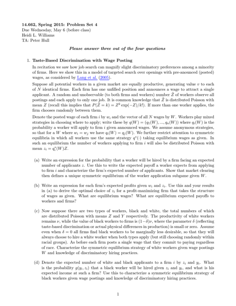
14.662, Spring 2015: Problem Set 4
Due Wednesday, May 6 (before class)
Heidi L. Williams
TA: Peter Hull
Please answer three out of the four questions
1. Taste-Based Discrimination with Wage Posting
In recitation we saw how job search can magnify slight discriminatory preferences among a minority
of firms. Here we show this in a model of targeted search over openings with pre-anounced (posted)
wages, as considered by Lang et al. (2005).
Suppose all potential workers in a given market are equally productive, generating value v to each
of N identical firms. Each firm has one unfilled position and announces a wage to attract a single
applicant. A random and unobservable (to both firms and workers) number Z̃ of workers observe all
postings and each apply to only one job. It is common knowledge that Z̃ is distributed Poisson with
mean Z (recall this implies that P (Z̃ = k) = Z k exp(−Z)/k!). If more than one worker applies, the
firm chooses randomly between them.
Denote the posted wage of each firm i by wi and the vector of all N wages by W . Workers play mixed
strategies in choosing where to apply; write these by q(W ) = (q1 (W ), ..., qn (W )) where qi (W ) is the
probability a worker will apply to firm i given announced wages. We assume anonymous strategies,
so that for a W where wi = wj we have qi (W ) = qj (W ). We further restrict attention to symmetric
equilibria in which all workers use the same strategy q ∗ (·) taking equilibrium wages as given. In
such an equilibrium the number of workers applying to firm i will also be distributed Poisson with
mean zi = qi∗ (W )Z.
(a) Write an expression for the probability that a worker will be hired by a firm facing an expected
number of applicants z. Use this to write the expected payoff a worker expects from applying
to firm i and characterize the firm’s expected number of applicants. Show that market clearing
then defines a unique symmetric equilibrium of the worker application subgame given W .
(b) Write an expression for each firm’s expected profits given wi and zi . Use this and your results
in (a) to derive the optimal choice of zi for a profit-maximizing firm that takes the structure
of wages as given. What are equilibrium wages? What are equilibrium expected payoffs to
workers and firms?
(c) Now suppose there are two types of workers, black and white, the total numbers of which
are distributed Poisson with means Z and Y respectively. The productivity of white workers
remains ν, while the value of black workers to firms is (1−δ)ν, where the parameter δ (reflecting
taste-based discrimination or actual physical differences in production) is small or zero. Assume
even when δ = 0 all firms find black workers to be marginally less desirable, so that they will
always choose to hire a white worker when both types apply (but still choosing randomly within
racial groups). As before each firm posts a single wage that they commit to paying regardless
of race. Characterize the symmetric equilibrium strategy of white workers given wage postings
W and knowledge of discriminatory hiring practices.
(d) Denote the expected number of white and black applicants to a firm i by zi and yi . What
is the probability g(yi , zi ) that a black worker will be hired given zi and yi , and what is his
expected income at such a firm? Use this to characterize a symmetric equilibrium strategy of
black workers given wage postings and knowledge of discriminatory hiring practices.
1
(e) Write an expression for expected firm profits given wi , zi , and yi . Using your expressions for
the expected earnings of white and black workers, derive and sign an expression for ∂zi /∂wi +
∂yi /∂wi , the marginal change in the expected number of job applicants given an increase in
wages. For arbitrarily small δ, argue that in equilibrium some firms will only attract whites
(“white firms”) while others will only attract blacks (“black firms”). Discuss.
(f) Let Nz and Ny be the numbers of white and black firms with rz ≡ Z/Nz and ry ≡ Y /Ny denot­
ing the expected number of applicants to each type of firm. Write expressions for equilibrium
wages and expected profits of white firms and the expected income of white workers. Argue
that equilibrium wages for black firms will be set at the expected income of white workers given
arbitrarily small δ. Use this to derive expressions for the expected income of black workers and
profits of black firms. Describe the discriminatory equilibrium. Are black workers unambigu­
ously worse off than white workers? How does the expected income of white and black workers
compare to the model without discrimination?
2
2. Wage Discrimination with Endogenous Human Capital Investment
Many of the models we’ve seen take groups’ human capital investments as given and analyze the
implications for wage disparities. Lundberg and Startz (1983) develop a model in which workers
anticipate wage setting practices in making their human capital investments. Here you’ll analyze
the implications of such “endogenous discrimination” for the observed skill/wage distribution.
Let πi denote the productivity of worker i, which depends on innate ability ai and acquired skill Xi .
πi = ai + bXi
Such skill is acquired at cost
c (Xi ) =
c
Xi2
2
for c > 0. Both workers and employers know the values of b and c, but employers do not observe
true productivity. Instead, they observe test scores that measure productivity with independent
error Ei .
T i = π i + εi
Both workers and employers know ai and εi are normally distributed with means ā and ε̄ and with
variances σa2 , and σε2 .
(a) How much training would workers purchase if employers could observe productivity directly?
What would be the equilibrium expense on training in this case?
(b) Solve for the equilibrium wage schedule under imperfect information. Start by assuming the
optimal level of training for worker i may be written as a linear function of ai and εi :
Xi = ρ0 + ρa ai + ρε εi
i. Use this expression to derive employers’ wage offers wi in terms of observed test scores Ti
the mean test score T¯, and mean productivity π̄.
ii. Taking this wage schedule as given, solve for the level of training that worker i acquires
and interpret your result.
iii. Use your results from (i) and (ii) to derive a new expression for the wage schedule as a
function of individual worker characteristics ai and εi . Interpret your result.
(c) Now suppose that workers belong to two observable groups. The groups have identical mean
innate characteristics ā and ε̄ and test variance σT2 , but group 1 has relatively heterogeneous
2 > σ 2 and σ 2 < σ 2
innate ability and relatively homogenous testing ability. Formally, σa,1
a,2
ε,1
ε,2
for groups 1 and 2. Repeat part (b), this time allowing the wage schedules to differ by group.
How much training does a worker in each group receive and what is her wage?
(d) Compare average wages for the two groups. Is this a discriminatory equilibrium by the Aigner
and Cain standard? Why do Lundberg and Startz consider it discriminatory?
(e) Now suppose that employers are prohibited from offering group-specific wage schedules. Let
f (εi , Ti ) denote the joint density of test-specific ability and test scores, and let f1 and f2
3
denote the corresponding group-specific densities. Let α denote the population fraction of
group 1 workers so that
f (εi , Ti ) = αf1 (εi , Ti ) + (1 − α)f2 (εi , Ti )
i. Assume that the equilibrium wage schedule will be linear in Ti , as in part (b), and let β
denote the coefficient on Ti so that wi = γ + βTi for some γ and β. Derive the optimal
level of human capital investment as a function of β. Use your result to argue that f1 and
f2 are bivariate normal.
ii. Derive an expression for f (εi | Ti ) and use it to derive the new wage schedule.
iii. How do average wages for the two groups compare now? Is this equilibrium discriminatory
by the Aigner and Cain standard? By Lundberg and Startz’s definition?
(f) Compare the total amount of training obtained under each equilibrium.
• Perfect information
• Imperfect information with group-specific wages
• Imperfect information with a common wage schedule
How does the ban on group-specific wages affect social welfare? Why?
4
3. Intergenerational Mobility
Consider a modified formalization of the Becker and Tomes (1979) model that we covered in class.
Family i consists of a parent of generation t − 1 that allocates earnings yi,t−1 between consumption
Ci,t−1 and investment Ii,t−1 in the human capital of her child of generation t. The investment
technology is given by
hit = δ + θ ln Ii,t−1 + eit
for θ > 0 and other sources of human capital (including genetics or cultural inheritance) eit . As
with Becker and Tomes (1979) suppose eit is first-order autoregressive:
eit = λei,t−1 + νit
for λ ∈ (0, 1) and a white noise error term νit . The child’s lifetime income is given by
ln yit = µ + ρhit
where ρ > 0 denotes the returns to human capital investment.
(a) Suppose parental utility is Cobb-Douglas in consumption and childhood earnings:
1−α α
Ui,t−1 = Ci,t−1
yit
Derive the optimal level of human capital investment and interpret.
(b) Write an expression linking ln yit and ln yi,t−1 . Can a standard intergenerational income re­
gression recover this relationship? Derive an expression (in terms of ρ, θ, and λ) for the
intergenerational income elasticity coefficient produced under this model. Discuss.
(c) Suppose we have data on three generations of individuals: t (children), t − 1 (parents), and
t − 2 (grandparents). Write an expression relating ln yit to ln yi,t−1 and ln yi,t−2 . Becker and
Tomes (1979) were the first to note that in a regression of these variables the coefficient on log
grandparent income can be negative (though small). A naı̈ve observer of this fact might take
this as refutation of a model where parents invest altruistically in their children. What is the
correct interpretation of this finding?
(d) Now suppose endowments are more persistent across generations; that is, suppose eit evolves
as
eit = λ1 ei,t−1 + λ2 ei,t−2 + νit
for 0 ≤ λ2 < λ1 < 1. Write an equation linking a child’s log income to his parent’s, grandpar­
ent’s, and great-grandparent’s. How might the availability of great-grandparent income data
update your priors on the parameters?
5
4. Early Life Determinants of Long-Run Outcomes
Deming (2009) is interested (in part) in estimating the effect of Head Start participation on later
student test scores. Participation in Head Start, however, is non-random. Altonji, Elder and Taber
(2005) provide a framework for thinking about the magnitude of bias induced by selection.
(a) Using the dataset provided, estimate the effect of Head Start participation on standardized
test scores, conditional on year fixed effects and the covariates provided in the dataset. Report
your estimate of the effect of Head Start. Discuss some reasons you might expect this estimate
to be biased.
(b) Now we will think about the process of selection into Head Start. Suppose that we can write
the following structural equation:
Y ∗ = αHS + W ' Γ
= αHS + X ' γ + E
Here, α is the true causal effect of Head Start on test scores Y ∗ . W is the full set of variables
(observed and unobserved) that determine Y ∗ along with HS, and Γ is the causal effect of
W on Y ∗ . X is a vector of the observable components of W , and γ and E are defined so that
Cov(X, E) = 0. These same X’s may influence whether a student participates in Head Start.
Write:
˜
HS = X ' β + HS
˜ is the residual.
where X ' β is the predicted value of HS from a regression of HS on X and HS
Show that the coefficient on HS from a regression of Y ∗ on HS and X can be expressed as:
α̃ = α +
V ar(HS)
(E(E|HS = 1) − E(E|HS = 0))
˜
V ar(HS)
Which parts of this expression are observable? Which are not?
(c) Assume the following variant of Condition 4 in Altonji, Elder and Taber (2005):
E[E|HS = 1] − E[E|HS = 0]
E[X ' γ|HS = 1] − E[X ' γ|HS = 0]
=K
V ar(E)
V ar(X ' γ)
Describe intuitively what the term K is. Under the null that Head Start has no impact (i.e.
α = 0), derive an expression for α̃ that depends only on K and observables. Assume (without
loss) that V ar(E) = 1.
(d) Use your expression in part (c) to estimate K. How large would selection on unobservables
relative to selection on observables have to be in order for the estimated effect of Head Start to
come entirely from selection? Be sure to think carefully about how the covariates you include
in X affect the sign of your estimates.
6
References
Altonji, Joseph, Todd Elder, and Christopher Taber, “Selection on observed and unobserved variables:
Assessing the effectiveness of Catholic schools,” Journal of Political Economy, 2005, 113 (1), 151–184. 4, 4c
Becker, Gary and Nigel Tomes, “An equilibrium theory of the distribution of income and intergenerational
mobility,” Journal of Political Economy, 1979, 87 (6), 1153–1189. 3, 3c
Deming, David, “Early childhood intervention and life-cycle skill development,” American Economic Journal:
Applied Economics, 2009, 1 (3), 111–134. 4
Lang, Kevin, Michael Manove, and William Dickens, “Racial discriminaiton in labor markets with posted
wage offers,” American Economic Review, 2005, 95 (4), 1327–1340. 1
Lundberg, Shelly and Richard Startz, “Private discrimination and social intervention in competitive labor
markets,” American Economic Review, 1983, 73 (3), 340–3347. 2
7
MIT OpenCourseWare
http://ocw.mit.edu
14.662 Labor Economics II
Spring 2015
For information about citing these materials or our Terms of Use, visit: http://ocw.mit.edu/terms.