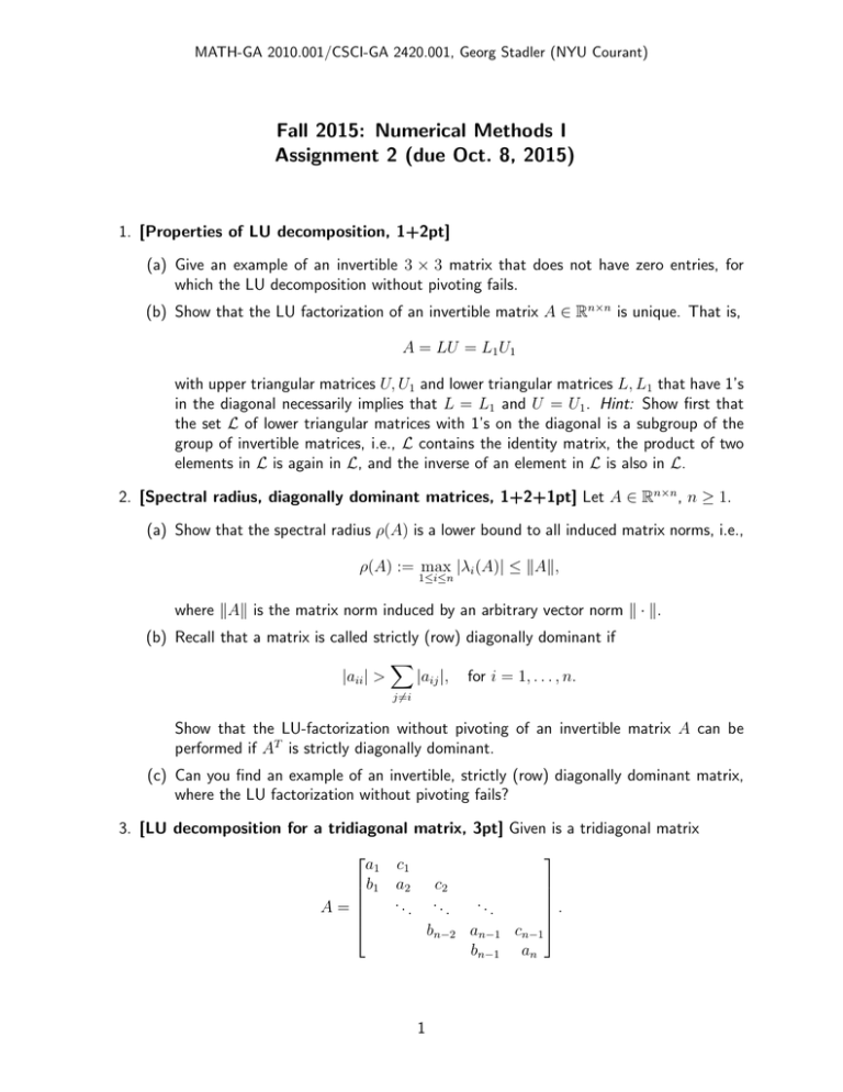
MATH-GA 2010.001/CSCI-GA 2420.001, Georg Stadler (NYU Courant)
Fall 2015: Numerical Methods I
Assignment 2 (due Oct. 8, 2015)
1. [Properties of LU decomposition, 1+2pt]
(a) Give an example of an invertible 3 × 3 matrix that does not have zero entries, for
which the LU decomposition without pivoting fails.
(b) Show that the LU factorization of an invertible matrix A ∈ Rn×n is unique. That is,
A = LU = L1 U1
with upper triangular matrices U, U1 and lower triangular matrices L, L1 that have 1’s
in the diagonal necessarily implies that L = L1 and U = U1 . Hint: Show first that
the set L of lower triangular matrices with 1’s on the diagonal is a subgroup of the
group of invertible matrices, i.e., L contains the identity matrix, the product of two
elements in L is again in L, and the inverse of an element in L is also in L.
2. [Spectral radius, diagonally dominant matrices, 1+2+1pt] Let A ∈ Rn×n , n ≥ 1.
(a) Show that the spectral radius ρ(A) is a lower bound to all induced matrix norms, i.e.,
ρ(A) := max |λi (A)| ≤ kAk,
1≤i≤n
where kAk is the matrix norm induced by an arbitrary vector norm k · k.
(b) Recall that a matrix is called strictly (row) diagonally dominant if
X
|aii | >
|aij |, for i = 1, . . . , n.
j6=i
Show that the LU-factorization without pivoting of an invertible matrix A can be
performed if AT is strictly diagonally dominant.
(c) Can you find an example of an invertible, strictly (row) diagonally dominant matrix,
where the LU factorization without pivoting fails?
3. [LU decomposition for a tridiagonal matrix, 3pt] Given is a tridiagonal matrix


a1 c 1
 b 1 a2 c 2



.
.
.

.
..
..
..
A=


bn−2 an−1 cn−1 
bn−1 an
1
Assuming that A has an LU decomposition, i.e., A = LU with




1
e 1 f1
..
..
d1 1



.
.
, U = 
,
L=
.
.



..
..
en−1 fn−1 
dn−1 1
en
derive recursive expressions for di , ei and fi .
4. [Forward substitution, 5pt] We implement forward substitution to solve the triangular
system
Lx = b,
where L ∈ Rn×n is an invertible, lower triangular matrix, and x, b ∈ Rn . Write functions
that take L and b as input arguments and return the solution x, and hand in code listings
with your assignment.
• Implement a naive forward substitution x = forward1(L,b) by looping over rows
(outer loop) and over columns (inner loop) (compare with Program 1 in Section 3.2.1
of Quarteroni/Sacci/Saleri, where the inner operation is replaced by looping over
columns).
• Implement forward substitution x = forward2(L,b) by looping over the rows (compare with class notes and Program 1 in Section 3.2.1 of Quarteroni/Sacci/Saleri).
• Implement forward substitution x = forward3(L,b) by looping over the columns
(compare with class notes and Program 2 in Section 3.2.1 of Quarteroni/Sacci/Saleri).
Choose a lower triangular matrix with random entries to verify that your implementations
are correct by comparing solutions with the build-in solver. Report timings for large systems (n = 10, 000 and larger) for each of your implementation as well as the build-in
implementation for solving linear systems (\ in MATLAB).1
5. [Implementing Choleski, 3+2pt] Implement the Choleski decomposition for a symmetric
and positive definite (spd) matrix A. The function C = mychol(A,b) should terminate if
it encounters a zero or negative diagonal element, and otherwise return the upper triangular
Choleski factor C such that A = C 0 C.
• Verify your implementation by comparing with the build-in Choleski factorization.
Document that comparison and hand in a code listing of mychol().
• Report timings for large (e.g., n = 500, 1000, 5000, 10000) spd matrices for your own
as well as the build-in Choleski factorization.2 Do the timings grow as expected from
floating point operation counts?
1
Despite the fact that each method requires roughly the same number of floating point operations, timings
should differ significantly. This is mainly due to memory access and how matrices are stored in memory. MATLAB
stores matrices as one-dimensional arrays, column by column. You can see that by accessing matrices with only
one index, i.e., using A(k) for an n×n matrix returns the entry A(m, l), where k = m+(l−1)n, 1 ≤ l, 1 ≤ m ≤ n.
Numbers that are next to each other in memory can be read from memory much faster than numbers that are
stored further away from each other.
2
You can generate a random spd matrix by multiplying a matrix with random entries with its transpose. The
resulting matrix is symmetric and positive semidefinite, and almost always positive definite.
2
6. [Sherman-Morrison formula, 6pt] Sometimes, one has to solve linear systems that are
rank-1 modifications of other linear systems, for which a factorization is already available.
Let us derive a solution algorithm for the modified system. Let A ∈ Rn×n be invertible and
u, v ∈ Rn be column vectors.
(a) Show that the matrix A + uv T is invertible if and only if v T Au 6= −1, and that in
this case the inverse is
(A + uv T )−1 = A−1 −
1
1+
v T A−1 u
A−1 uv T A−1 .
(b) Let v T A−1 u 6= −1 and assume given the LU decomposition of A. Specify an efficient algorithms based on the Sherman-Morrison formula to solve the rank-1 modified
system (A + uv T )x = b for a given right hand side b ∈ Rn .
(c) Use the above algorithm to solve the system
 


16
2 2 3 4 5
32
2 6 6 8 10
 


3 6 10 12 15 x = 46
 


62
4 8 12 18 20
80
5 10 15 20 30
by choosing a proper diagonal matrix for A.
7. [Iterative solution of linear systems, 6pt] Let us study iterative solvers for linear systems
Ax = b, where A ∈ Rn×n and x, b ∈ Rn . For every n, A and b have the same structure,
for instance for n = 7:

 

0 0 3 −1 0 0 0
1
 0 0 −1 3 −1 0 0 
1

 

 0 0 0 −1 3 −1 0 
1

 

1 .
,
0
0
0
0
−1
3
−1
A=
b
=

 

−1 0 0 0 0 −1 3 
1

 

 3 −1 0 0 0 0 −1
1
1
−1 3 0 0 0 0 0
(a) Why is it not possible to apply the Jacobi or the Gauss-Seidel iteration for solving
this linear system directly? Which rows/columns must be exchanged such that the
resulting linear system can be solved with these methods? In the following, we always
consider the system with properly exchanged rows/columns.
(b) Argue why the Jacobi and the Gauss Seidel method converge.
(c) Specify the iteration for the Jacobi and the Gauss-Seidel iteration component-wise.
(d) Implement both methods using component-wise expressions—you should never have
to assemble a matrix. Apply your implementation for the solution of the problem for
n = 102 , 103 , 104 , and report the number of iterations for each n for both methods.
Use x0 = 0 as initialization, and terminate the iteration when the norm of the residual
3
r k := b − Axk has decreased by a factor of 108 compared to the initial residual r 0 ,
i.e., when
kr k k
< 10−8 .
kr 0 k
8. [Solving without explicit knowledge of system matrix, up to 4pt extra credit3 ] As
mentioned in class, it can happen that one needs to solve a linear system of the form
Ax = b,
where the entries of A are not available explicitly, but we can apply A to vectors. Imagine
we only have a function Afun, which applies the matrix A to vectors, i.e., Afun(x) = Ax.4
Being able to apply the matrix to vectors can, in principle, be used to assemble the matrix A
(How?), but this is often inefficient or infeasible. In such a case, factorization-based solvers
cannot be used and we must rely on iterative solvers, for instance the Jacobi method.
(a) I provide you with a function Afun()5 corresponding to a linear matrix A. The
function corresponds to the discretization of a differential operator, and can be applied
to vectors of length N 2 , where N ∈ N—that is, the underlying matrix is of size
N 2 × N 2 . We know that the diagonal entries of the underlying matrix A are all equal
to 4(N + 1)2 , and that the matrix is symmetric and positive definite. Experiment with
the Jacobi method to solve the system for N = 50, where the right hand side b is a
vector of all ones.
(b) Try to find the optimal damping parameter for the Jacobi method.6 Compare the
number of iterations required to achieve a tolerance without damping and with the
optimal damping parameter.
(c) An important iterative solver for symmetric positive definite linear systems in the
conjugate gradient (CG) method. Similarly to the Jacobi method, CG also only
requires a function Afun rather than the explicit matrix. Moreover, CG does not
even require knowledge of the diagonal of A.7 Solve the linear system using CG and
compare the number of iterations with the Jacobi method.8
3
Please only attempt this problem if you are interested in it and not for the extra points; the problem is meant
to give you more freedom and allow you to explore aspects of iterative solvers.
4
This can happen, for instance, if A involves a sequence of linear matrix applications and solves and it would
be very inefficient to multiply out all these operations, of if A involves linear operations for which fast algorithms
(e.g., the fast Fourier transform (FFT) or the fast multipole method (FMM)) are available.
5
Download the MATLAB function from http://cims.nyu.edu/~stadler/num1/material/Afun.m.
6
This will require an estimate of smallest and largest eigenvalues. MATLAB provides the function eigs for
estimating eigenvalues of large matrices that are not available explicitly. Use help eigs to learn more.
7
Learn about MATLAB’s CG implementation pcg by reading the corresponding help pages. We will not have
much time to cover the CG method in class, but it is one of the most important iterative solvers, and an important
member of the family of so-called Krylov subspace methods.
8
Each iteration of CG requires one call to Afun, i.e., one application of A to a vector. The same is true for
the Jacobi method, and usually the computation of Ax is the most expensive part of the algorithms. Thus, the
cost per CG and Jacobi iteration is similar, and one can just compare the iterations numbers.
4