Research Journal of Applied Sciences, Engineering and Technology 10(1): 22-28,... ISSN: 2040-7459; e-ISSN: 2040-7467

Research Journal of Applied Sciences, Engineering and Technology 10(1): 22-28, 2015 ISSN: 2040-7459; e-ISSN: 2040-7467 © Maxwell Scientific Organization, 2015 Submitted: ‎ November ‎10, ‎2014 Accepted: February ‎8, ‎2015 Published: May 10, 2015 Bayesian Estimation of a Mixture Model Ilhem Merah and Assia Chadli Probability and Statistics Laboratory, Badji Mokhtar University, BP12, Annaba 23000, Algeria Abstract: We present the properties of a bathtub curve reliability model having both a sufficient adaptability and a minimal number of parameters introduced by Idée and Pierrat (2010). This one is a mixture of a Gamma distribution G(2, (1/θ)) and a new distribution L(θ). We are interesting by Bayesian estimation of the parameters and survival function of this model with a squared-error loss function and non-informative prior using the approximations of Lindley (1980) and Tierney and Kadane (1986). Using a statistical sample of 60 failure data relative to a technical device, we illustrate the results derived. Based on a simulation study, comparisons are made between these two methods and the maximum likelihood method of this two parameters model. Keywords: Approximations, bayes estimator, mixture distribution, reliability, weibull distribution INTRODUCTION Pierrat (2010). These authors showed that this model of two parameters is equivalent to a mixture of two Weibull distributions. Equivalence was shown using Kolmogorov Smirnov distance. We propose to use a Bayesian approach, with a non-informative prior and a squared-error loss function. The main objective of this study is to estimate the two parameters and the survival function of the new model. The methods under consideration are: Maximum likelihood Estimation, Bayesian Methods with two types of approximation: Lindley's approximation and Tierney-Kadane's approximation. The methods are compared using a real data analysis and simulation. Conclusions based on the study are given. Mixture models play a vital role in many applications. For example, direct applications of finite mixture models are in economics, botany, medicine, psychology, agriculture, zoology, life testing and reliability engineering. However, a modelling by a finished mixture of Weibull distributions can be more relevant and physically significant. Several authors are interesting by Bayesian estimation in mixture models like Tsionas (2002) and Gelman et al. (2003). Modelling by a Weibull mixture distributions was often occulted by the survival analysis experts to the profile of a simple model of Weibull, because of the high number of parameters to be estimated and absence of an effective estimation method of the parameters. Several methods are used for estimating the parameters of the mixture. The graphic approach was used by Jiang and Murty (1995) and Jiang and Kececioglu (1992) initially to adjust data with a mixture of two Weibull distributions, then to estimate its parameters. The two methods of the moments and the maximum likelihood were largely used while being based on the use of EM algorithm (ExpectationMaximization), this algorithm is not only one digital technique, it gives also useful statistical data, for more detail to see Dempster et al. (1977). A modification of this algorithm was introduced by Wei and Tanner (1990), where in the step E, the expectation is calculated by Monte Carlo simulations, this algorithm noted MCEM was used by Levine and Casella (2001) and more recently by Elmahdy and Aboutahoun (2013). 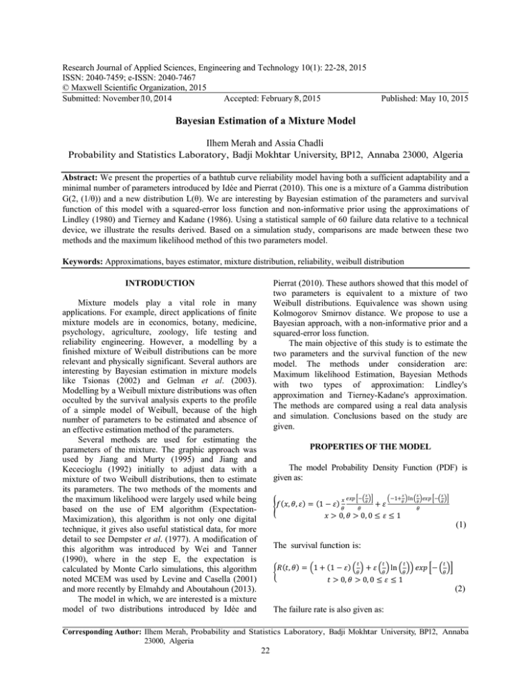The model in which, we are interested is a mixture model of two distributions introduced by Idée and PROPERTIES OF THE MODEL The model Probability Density Function (PDF) is given as: 𝑥𝑥 𝑥𝑥 𝑥𝑥 𝑒𝑒𝑒𝑒𝑒𝑒 �−� �� 𝑥𝑥 𝜃𝜃 𝑥𝑥 𝜃𝜃 �−1+ � ln � �𝑒𝑒𝑒𝑒𝑒𝑒 �−� �� 𝜃𝜃 𝜃𝜃 + 𝜀𝜀 �𝑓𝑓(𝑥𝑥, 𝜃𝜃, 𝜀𝜀) = (1 − 𝜀𝜀) 𝜃𝜃 𝜃𝜃 𝑥𝑥 > 0, 𝜃𝜃 > 0, 0 ≤ 𝜀𝜀 ≤ 1 𝜃𝜃 (1) The survival function is: � 𝑡𝑡 𝑡𝑡 𝑡𝑡 𝑡𝑡 𝑅𝑅(𝑡𝑡, 𝜃𝜃) = �1 + (1 − 𝜀𝜀) � � + 𝜀𝜀 � � ln � �� 𝑒𝑒𝑒𝑒𝑒𝑒 �− � �� 𝜃𝜃 𝜃𝜃 𝜃𝜃 𝜃𝜃 𝑡𝑡 > 0, 𝜃𝜃 > 0, 0 ≤ 𝜀𝜀 ≤ 1 (2) The failure rate is also given as: Corresponding Author: Ilhem Merah, Probability and Statistics Laboratory, Badji Mokhtar University, BP12, Annaba 23000, Algeria 22 Res. J. Appl. Sci. Eng. Technol., 10(1): 22-28, 2015 𝑡𝑡 1+𝜀𝜀 ln � � 1 𝜃𝜃 ℎ(𝑡𝑡, 𝜀𝜀, 𝜃𝜃) = �1 − 𝑡𝑡 𝑡𝑡 𝑡𝑡 � 𝜃𝜃 � 1+(1−𝜀𝜀)� �+𝜀𝜀� � ln � � 𝜃𝜃 𝜃𝜃 𝜃𝜃 𝑡𝑡 > 0, 𝜃𝜃 > 0, 0 ≤ 𝜀𝜀 ≤ 1 (3) 𝑙𝑙(𝜃𝜃, 𝜀𝜀/𝑒𝑒𝑒𝑒ℎ) = 𝜃𝜃 𝜃𝜃 𝑛𝑛 𝑥𝑥 𝑖𝑖 𝑥𝑥 𝑖𝑖 ∏𝑛𝑛𝑖𝑖=1 𝑥𝑥 𝑖𝑖 �(1 − 𝜀𝜀) � � + 𝜀𝜀 � − 1� ln � �� 𝜃𝜃 We pose: 𝜃𝜃 𝜋𝜋(𝜀𝜀, 𝜃𝜃) = 𝑆𝑆 𝑒𝑒𝑒𝑒𝑒𝑒 �−� �� 𝜃𝜃 𝜃𝜃 𝜃𝜃 𝜃𝜃 𝜀𝜀̂ = Then: 𝑙𝑙(𝜃𝜃, 𝜀𝜀/𝑒𝑒𝑒𝑒ℎ) = 𝑆𝑆 𝑒𝑒𝑒𝑒𝑒𝑒 �− ∑𝑛𝑛𝑖𝑖=1 � 𝜃𝜃 𝜃𝜃 𝑛𝑛 The log- likelihood is: ∏𝑛𝑛𝑖𝑖=1�𝑢𝑢𝑖𝑖 (𝜀𝜀, 𝜃𝜃)� 𝑆𝑆 𝐿𝐿(𝜃𝜃, 𝜀𝜀/𝑒𝑒𝑒𝑒ℎ) = −𝑛𝑛 ln(𝜃𝜃) − + ∑𝑛𝑛𝑖𝑖=1 ln(𝑢𝑢𝑖𝑖 ) 𝜃𝜃 𝜕𝜕𝜕𝜕 𝜕𝜕𝜕𝜕 𝜕𝜕𝜕𝜕 𝑆𝑆 = − 𝑛𝑛 + ∑𝑛𝑛𝑖𝑖=1 � 𝜃𝜃 = −𝑥𝑥 ∑𝑛𝑛𝑖𝑖=1 � 𝑖𝑖 𝜃𝜃 −𝑥𝑥 𝑖𝑖 +𝜀𝜀𝜀𝜀 𝑥𝑥 𝑖𝑖 𝜃𝜃 +� − 𝜃𝜃 𝑥𝑥 From where, we obtain this system: 𝑆𝑆 𝜃𝜃 � − 𝑛𝑛 + ∑𝑛𝑛𝑖𝑖=1 � ∑𝑛𝑛𝑖𝑖=1 � −𝑥𝑥 𝑖𝑖 𝜃𝜃 −𝑥𝑥 𝑖𝑖 +𝜀𝜀𝜀𝜀 𝜃𝜃 𝑥𝑥 𝑥𝑥 =0 𝑥𝑥 ∞ 1 𝜃𝜃 𝑆𝑆 ∞ 1 𝑒𝑒𝑒𝑒𝑒𝑒 �−�𝜃𝜃 �� 𝑛𝑛 ∏𝑖𝑖=1 �𝑢𝑢 𝑖𝑖 (𝜀𝜀,𝜃𝜃)�𝑑𝑑𝑑𝑑𝑑𝑑𝑑𝑑 ∫0 𝜀𝜀𝜃𝜃 𝑛𝑛 ∞ 1 ∫0 ∫0 𝑙𝑙(𝜃𝜃,𝜀𝜀/𝑒𝑒𝑒𝑒ℎ)𝜋𝜋(𝜀𝜀,𝜃𝜃)𝑑𝑑𝑑𝑑𝑑𝑑𝑑𝑑 𝑡𝑡 𝑡𝑡 𝑆𝑆 𝑡𝑡 𝑒𝑒𝑒𝑒𝑒𝑒 �−�𝜃𝜃 �� 𝑛𝑛 ∏𝑖𝑖=1 �𝑢𝑢 𝑖𝑖 (𝜀𝜀,𝜃𝜃)�𝑑𝑑𝑑𝑑𝑑𝑑𝑑𝑑 𝜀𝜀𝜃𝜃 𝑛𝑛 +1 𝑆𝑆 ∞ 1 𝑒𝑒𝑒𝑒𝑒𝑒 �−�𝜃𝜃 �� 𝑛𝑛 ∏𝑖𝑖=1�𝑢𝑢 𝑖𝑖 (𝜀𝜀,𝜃𝜃)�𝑑𝑑𝑑𝑑𝑑𝑑𝑑𝑑 𝜀𝜀𝜃𝜃 𝑛𝑛 +1 To solve this ratio of integrals explicitly, we will use approximation methods. (7) Lindley’s procedure: Lindley (1980) developed approximate procedures for the evaluation of the ratio of integrals of the form: 𝑥𝑥 𝜃𝜃 ∫ 𝑤𝑤(𝜃𝜃)𝑒𝑒𝑒𝑒𝑒𝑒 {𝐿𝐿(𝜃𝜃)}𝑑𝑑𝑑𝑑 ∫ 𝑣𝑣(𝜃𝜃)𝑒𝑒𝑒𝑒𝑒𝑒 {𝐿𝐿(𝜃𝜃)}𝑑𝑑𝑑𝑑 (9) In our case, 𝑚𝑚 = 2 and 𝜆𝜆 = (𝜀𝜀, 𝜃𝜃) 𝜌𝜌(𝜀𝜀, 𝜃𝜃) = log{𝜋𝜋(𝜀𝜀, 𝜃𝜃)} ʌ(𝜀𝜀, 𝜃𝜃) = log{𝜋𝜋(𝜀𝜀, 𝜃𝜃|𝑥𝑥)} = 𝐿𝐿(𝜀𝜀, 𝜃𝜃) + 𝜌𝜌(𝜀𝜀, 𝜃𝜃) = 𝑆𝑆 = − ln(𝜀𝜀𝜀𝜀) − 𝑛𝑛 ln(𝜃𝜃) − + ∑𝑛𝑛𝑖𝑖=1 ln�𝑢𝑢𝑖𝑖 (𝜀𝜀, 𝜃𝜃)� 𝜃𝜃 (10) Denoting 𝛷𝛷(𝑡𝑡) = 𝑅𝑅𝑡𝑡 and using Lindley's method, expanding about the posterior mode, the Bayesian estimator of 𝑅𝑅𝑡𝑡 in Eq. (2) becomes: The resolution of the system is done using the iterative methods and provides us estimators of the maximum of likelihood of 𝜃𝜃 and 𝜀𝜀 noted respectively by 𝜃𝜃𝑀𝑀𝑀𝑀 and 𝜀𝜀𝑀𝑀𝑀𝑀 . To have an estimator of the survival function, it is enough to replace (𝜀𝜀, 𝜃𝜃) in the expression (2) by (𝜃𝜃𝑀𝑀𝑀𝑀 , 𝜀𝜀𝑀𝑀𝑀𝑀 ), we obtain an estimator of the survival function noted 𝑅𝑅𝑀𝑀𝑀𝑀 (𝑡𝑡). Bayesian estimation: Given a random sample, (𝑥𝑥1 , 𝑥𝑥2 , … , 𝑥𝑥𝑛𝑛 ) of size n, from a mixture distribution and ⨱ the vector of the observed data. The likelihood function can be constructed as follows: 𝑡𝑡 ∫0 ∫0 + � 𝑖𝑖 − 1� ln � 𝑖𝑖 �� 𝑢𝑢𝑖𝑖−1 = 0 𝜃𝜃 𝑆𝑆 ∞ 1 𝑒𝑒𝑒𝑒𝑒𝑒 �−�𝜃𝜃 �� 𝑛𝑛 ∏𝑖𝑖=1�𝑢𝑢 𝑖𝑖 (𝜀𝜀,𝜃𝜃)�𝑑𝑑𝑑𝑑𝑑𝑑𝑑𝑑 𝑛𝑛 +1 𝜃𝜃 ∞ 1 𝜀𝜀 ∫0 ∫0 𝑙𝑙�𝜃𝜃,𝑒𝑒𝑒𝑒 ℎ �𝜋𝜋(𝜀𝜀,𝜃𝜃)𝑑𝑑𝑑𝑑𝑑𝑑𝑑𝑑 ∫0 ∫0 �1+(1−𝜀𝜀)𝜃𝜃 +𝜀𝜀 𝜃𝜃 ln �𝜃𝜃 ��𝑒𝑒𝑒𝑒𝑒𝑒 �−𝜃𝜃 � − 𝜀𝜀 � 𝑖𝑖 � ln � 𝑖𝑖 �� 𝑢𝑢𝑖𝑖−1 = 0, 𝜃𝜃 (8) ∫0 ∫0 𝑅𝑅𝑡𝑡∗ = 𝐸𝐸(𝑅𝑅𝑡𝑡 |𝑥𝑥 ) 𝑥𝑥 1� ln � �� 𝑢𝑢𝑖𝑖−1 𝜃𝜃 ∏𝑛𝑛𝑖𝑖=1�𝑢𝑢𝑖𝑖 (𝜀𝜀, 𝜃𝜃)� ∝ The Bayesian estimator of 𝑅𝑅𝑡𝑡 under the loss function is the posterior mean: (5) − 𝜀𝜀 � 𝑖𝑖 � ln � 𝑖𝑖 �� 𝑢𝑢𝑖𝑖−1 = 0 𝜃𝜃 𝜃𝜃 (6) 𝑥𝑥 𝑖𝑖 𝑙𝑙(𝜃𝜃,𝜀𝜀/𝑒𝑒𝑒𝑒ℎ)𝜋𝜋(𝜀𝜀,𝜃𝜃) ∫ 𝜃𝜃� = 0 Differentiating (5) with respect to 𝜀𝜀 and 𝜃𝜃 and equating to zero, we have: 𝜕𝜕𝜕𝜕 ∞ 1 ∫0 ∫0 𝑙𝑙(𝜃𝜃,𝜀𝜀/𝑒𝑒𝑒𝑒ℎ)𝜋𝜋(𝜀𝜀,𝜃𝜃)𝑑𝑑𝑑𝑑𝑑𝑑𝑑𝑑 The Bayesian estimates of parameters under the loss function are: 𝑥𝑥 𝑖𝑖 𝑢𝑢𝑖𝑖 (𝜀𝜀, 𝜃𝜃) = �(1 − 𝜀𝜀) � � + 𝜀𝜀 � − 1� ln � �� ; 𝑆𝑆 = ∑𝑛𝑛𝑖𝑖=1 𝑥𝑥𝑖𝑖 1 𝜀𝜀𝜀𝜀 𝜋𝜋(𝜀𝜀, 𝜃𝜃|⨱) = 𝜀𝜀𝜃𝜃 𝑛𝑛 +1 𝑥𝑥 𝑖𝑖 ∏𝑛𝑛𝑖𝑖=1�𝑢𝑢𝑖𝑖 (𝜀𝜀, 𝜃𝜃)� The posterior distribution is given by: (4) 𝜃𝜃 𝑥𝑥 𝑖𝑖 𝜃𝜃 𝑛𝑛 Using the non-informative prior: Maximum likelihood: We lay out of a sample of n independent and complete observations of the same distribution given in (1) noted (𝑥𝑥1 , 𝑥𝑥2 , … , 𝑥𝑥𝑛𝑛 ). The likelihood of the sample is written: 𝑥𝑥 𝑒𝑒𝑒𝑒𝑒𝑒 �− ∑𝑛𝑛𝑖𝑖=1� 𝑖𝑖 �� 𝑆𝑆 𝑒𝑒𝑒𝑒𝑒𝑒 �−� �� 𝜃𝜃 𝑙𝑙(𝜃𝜃, 𝜀𝜀/𝑒𝑒𝑒𝑒ℎ) = 23 1 1 𝑅𝑅𝑡𝑡∗ = 𝛷𝛷�𝜆𝜆̂� + ∑ 𝛷𝛷𝑖𝑖𝑖𝑖 �𝜆𝜆̂�𝜏𝜏𝑖𝑖𝑖𝑖 + ∑ ʌ𝑖𝑖𝑖𝑖𝑖𝑖 𝛷𝛷𝑙𝑙 �𝜆𝜆̂�𝜏𝜏𝑖𝑖𝑖𝑖 𝜏𝜏𝑘𝑘𝑘𝑘 (11) 2 2 Res. J. Appl. Sci. Eng. Technol., 10(1): 22-28, 2015 where, 𝜕𝜕 2 𝛷𝛷 𝛷𝛷𝑖𝑖𝑖𝑖 = 𝜕𝜕𝜆𝜆 𝑖𝑖 𝜕𝜕𝜆𝜆 𝑗𝑗 , ʌ𝑖𝑖𝑖𝑖𝑖𝑖 = 𝜕𝜕 3 ʌ 𝜕𝜕𝜆𝜆 𝑖𝑖 𝜕𝜕𝜆𝜆 𝑗𝑗 𝜕𝜕𝜆𝜆 𝑘𝑘 , 𝑒𝑒𝑒𝑒𝑒𝑒 ʌ222 = (12) The 𝜏𝜏𝑖𝑖𝑖𝑖 values are defined as the (𝑖𝑖, 𝑗𝑗)th element of the negative of the inverse of the Hessian matrix of −1 of ʌ: �𝜏𝜏𝑖𝑖𝑖𝑖 � = −�ʌ𝑖𝑖𝑖𝑖 � . signe second derivatives Expanding Eq. (7), we obtain: 1 𝑅𝑅𝐵𝐵∗ (𝑡𝑡) = 𝛷𝛷�𝜆𝜆̂� + 𝛷𝛷11 �𝜆𝜆̂�𝜏𝜏11 + 𝛷𝛷12 �𝜆𝜆̂�𝜏𝜏12 + 1 2 1 2 1 2 𝛷𝛷22 �𝜆𝜆̂�𝜏𝜏22 + ʌ111 �𝛷𝛷1 �𝜆𝜆̂�𝜏𝜏11 + 𝛷𝛷2 �𝜆𝜆̂�𝜏𝜏11 𝜏𝜏12 � + 2 ʌ112 = 2 )� ʌ �3𝛷𝛷1 �𝜆𝜆̂�𝜏𝜏11 𝜏𝜏12 + 𝛷𝛷2 �𝜆𝜆̂�(𝜏𝜏11 𝜏𝜏22 + 2𝜏𝜏12 + 2 112 1 2 1 2 2 )� ʌ122 �3𝛷𝛷2 �𝜆𝜆̂�𝜏𝜏22 𝜏𝜏12 + 𝛷𝛷1 �𝜆𝜆̂�(𝜏𝜏11 𝜏𝜏22 + 2𝜏𝜏12 + 2 ʌ222 �𝛷𝛷2 �𝜆𝜆̂�𝜏𝜏22 + 𝛷𝛷1 �𝜆𝜆̂�𝜏𝜏22 𝜏𝜏12 � (13) ʌ122 In our case, with 𝑚𝑚 = 2 and 𝜆𝜆 = (𝜀𝜀, 𝜃𝜃), we obtain from Eq. (2), with 𝛷𝛷(𝑡𝑡) = 𝑅𝑅𝑡𝑡 : 𝛷𝛷1 = 𝜕𝜕𝛷𝛷 𝜕𝜕𝜕𝜕 𝛷𝛷12 = 𝜕𝜕𝛷𝛷 𝜕𝜕𝜕𝜕 =� 𝑡𝑡 𝑡𝑡𝑡𝑡𝑡𝑡𝑡𝑡 �−� �� 𝜃𝜃 = 𝜕𝜕 2 𝛷𝛷 = 𝜕𝜕𝜕𝜕𝜕𝜕𝜕𝜕 𝑡𝑡𝑢𝑢 𝑡𝑡 𝛷𝛷22 = 𝜃𝜃 2 � 𝑒𝑒𝑒𝑒𝑒𝑒 �− � ��, 𝜕𝜕 2 𝛷𝛷 𝜕𝜕𝜃𝜃 2 = 𝜃𝜃 𝑡𝑡 𝜃𝜃 𝜃𝜃 2 𝑡𝑡 𝑡𝑡 �−1 + ln � �� , 𝛷𝛷11 = 𝜃𝜃 𝑡𝑡 𝑡𝑡𝑡𝑡𝑡𝑡𝑡𝑡 �−� �� 𝜃𝜃 𝑡𝑡 𝑡𝑡 2 𝑒𝑒𝑒𝑒𝑒𝑒 �−� �� 𝑡𝑡 𝜕𝜕 2 𝛷𝛷 𝑡𝑡 𝜕𝜕𝜀𝜀 2 = 0, �− + � − 1� ln � �� , 𝛷𝛷2 = 𝜃𝜃 𝜃𝜃 𝜃𝜃 𝜃𝜃 𝜀𝜀 � 𝑆𝑆 −(1 + 𝑛𝑛) + + ∑𝑛𝑛𝑖𝑖=1 𝑣𝑣𝑖𝑖 𝑢𝑢𝑖𝑖−1 = 0, 𝜃𝜃 The partial derivatives of the log-posterior density function are: ʌ22 = �𝑢𝑢𝑖𝑖−1 ʌ12 = 𝜕𝜕 2 ʌ 𝜕𝜕𝜃𝜃 2 = 1 𝜀𝜀 2 𝑙𝑙 = So that: + ∑𝑛𝑛𝑖𝑖=1(−𝑠𝑠𝑖𝑖2 𝑢𝑢𝑖𝑖−2 ), 1+𝑛𝑛 𝜃𝜃 2 − 2𝑆𝑆 𝜃𝜃 3 + ∑𝑛𝑛𝑖𝑖=1 2 𝜕𝜕𝜀𝜀 3 =− 2 𝜀𝜀 3 + 2 ∑𝑛𝑛𝑖𝑖=1 𝑠𝑠𝑖𝑖3 𝑢𝑢𝑖𝑖−3 , 𝜃𝜃 log 𝑣𝑣(𝜆𝜆)+𝐿𝐿(𝜆𝜆|𝑥𝑥 ) 𝑛𝑛 , 𝑙𝑙 ∗ = 𝜃𝜃 𝑥𝑥 𝑖𝑖 𝜃𝜃 + log 𝛷𝛷(𝜆𝜆)+log 𝑣𝑣(𝜆𝜆)+𝐿𝐿(𝜆𝜆|𝑥𝑥 ) 𝑛𝑛 ∫ 𝑒𝑒𝑒𝑒𝑒𝑒 (𝑛𝑛𝑙𝑙 ∗ )𝑑𝑑𝑑𝑑 . ∫ 𝑒𝑒𝑒𝑒𝑒𝑒 (𝑛𝑛𝑛𝑛 )𝑑𝑑𝑑𝑑 ∗ 𝑛𝑛 𝜕𝜕 3 ʌ 𝑥𝑥 𝑖𝑖 |𝛯𝛯 | 𝐸𝐸� (𝛷𝛷(𝜆𝜆)|𝑥𝑥 ) = � |𝛯𝛯| � 𝜕𝜕 2 ʌ 1 𝑥𝑥𝑖𝑖 𝑥𝑥𝑖𝑖 = � �𝑢𝑢𝑖𝑖−1 �1 − ln � �� − 𝑣𝑣𝑖𝑖 𝑠𝑠𝑖𝑖 𝑢𝑢𝑖𝑖−2 �, 𝜃𝜃 𝜃𝜃 𝜕𝜕𝜕𝜕𝜕𝜕𝜕𝜕 𝜃𝜃 ʌ111 = 𝑥𝑥 𝜃𝜃 , (14) (15) The Bayesian estimator of 𝛷𝛷(𝜆𝜆) takes the form: 2𝜀𝜀𝑥𝑥𝑖𝑖 𝑥𝑥𝑖𝑖 2𝑥𝑥𝑖𝑖 + 𝜀𝜀𝑥𝑥𝑖𝑖 − 𝜀𝜀𝜀𝜀 � ln � � + � − 𝑣𝑣𝑖𝑖2 𝑢𝑢𝑖𝑖−2 � 𝜃𝜃 𝜃𝜃 𝜃𝜃 𝑖𝑖=1 𝑥𝑥 � − 𝜀𝜀 � 𝑖𝑖 � ln � 𝑖𝑖 �;𝑠𝑠𝑖𝑖 = − 𝐸𝐸(𝛷𝛷(𝜆𝜆)|𝑥𝑥 ) = 1 𝜃𝜃 𝜃𝜃 Tierney and Kadane’s method: Lindley's approximation requires the evaluation of the third derivatives of the likelihood function or the posterior density which can be very tedious and requires great computational precision. Tierney and Kadane (1986) gave an alternative method of evaluation of the ratio of integrals, by writing the two expressions: 1 = −𝑥𝑥 𝑖𝑖 +𝜀𝜀𝜀𝜀 � − 1� ln � � − + ∑𝑛𝑛𝑖𝑖=1 𝑠𝑠𝑖𝑖 𝑢𝑢𝑖𝑖−1 = 0, 𝜕𝜕 2 ʌ 𝑛𝑛 𝑥𝑥 𝑖𝑖 With 𝛷𝛷(𝑡𝑡) = 𝑅𝑅𝑡𝑡 . The joint posterior mode of Eq. (10) is obtained by solving the system of equations: 𝜕𝜕𝜀𝜀 2 𝑖𝑖=1 + 𝑣𝑣𝑖𝑖 𝑠𝑠𝑖𝑖−2 𝑢𝑢𝑖𝑖−3 � , 𝜕𝜕 3 ʌ 1 𝑥𝑥𝑖𝑖 − 𝜃𝜃 2𝑥𝑥𝑖𝑖 𝑥𝑥𝑖𝑖 = = 2 � �𝑢𝑢𝑖𝑖−1 � + ln � �� 2 𝜕𝜕𝜕𝜕𝜕𝜕𝜃𝜃 𝜃𝜃 𝜃𝜃 𝜃𝜃 𝜃𝜃 𝑖𝑖=1 2𝜀𝜀𝑥𝑥 𝑥𝑥 𝑖𝑖 𝑖𝑖 − 𝑠𝑠𝑖𝑖 𝑢𝑢𝑖𝑖−2 � ln � � 𝜃𝜃 𝜃𝜃 2𝑥𝑥𝑖𝑖 + 𝜀𝜀𝑥𝑥𝑖𝑖 − 𝜀𝜀𝜀𝜀 � + 𝜃𝜃 𝑥𝑥𝑖𝑖 𝑥𝑥𝑖𝑖 −2 + 2𝑣𝑣𝑖𝑖 𝑢𝑢𝑖𝑖 �1 − ln � �� 𝜃𝜃 𝜃𝜃 2 −3 � + 2𝑠𝑠𝑖𝑖 𝑣𝑣𝑖𝑖 𝑢𝑢𝑖𝑖 𝑣𝑣𝑖𝑖 = � 𝜃𝜃𝜃𝜃 − 𝜃𝜃 − 4𝑡𝑡 + 3𝜀𝜀𝜀𝜀 2𝜃𝜃𝜃𝜃 𝑡𝑡 𝑡𝑡 �𝑢𝑢𝑡𝑡 + +� − 4𝜀𝜀� ln � �� + 3 𝛷𝛷(𝑡𝑡) 𝑡𝑡 𝑡𝑡 𝜃𝜃 𝜃𝜃 ʌ11 = 𝑛𝑛 𝜕𝜕 3 ʌ 2 𝑥𝑥𝑖𝑖 𝑥𝑥𝑖𝑖 = � �𝑠𝑠𝑖𝑖 𝑢𝑢𝑖𝑖−2 �1 − ln � �� 𝜕𝜕𝜀𝜀 2 𝜕𝜕𝜕𝜕 𝜃𝜃 𝜃𝜃 𝜃𝜃 where, 𝜃𝜃 𝜃𝜃 4 −2(𝑛𝑛 + 1) 6𝑆𝑆 + 4 𝜃𝜃 3 𝜃𝜃 𝑛𝑛 1 −6𝑥𝑥𝑖𝑖 + 2𝜀𝜀𝜀𝜀 − 5𝜀𝜀𝑥𝑥𝑖𝑖 + 3 � �𝑢𝑢𝑖𝑖−1 � 𝜃𝜃 𝜃𝜃 𝑖𝑖=1 𝑥𝑥𝑖𝑖 𝑥𝑥𝑖𝑖 − 6𝜀𝜀 ln � �� 𝜃𝜃 𝜃𝜃 2𝜀𝜀𝑥𝑥𝑖𝑖 𝑥𝑥𝑖𝑖 −2 − 3𝑣𝑣𝑖𝑖 𝑢𝑢𝑖𝑖 � ln � � 𝜃𝜃 𝜃𝜃 2𝑥𝑥𝑖𝑖 + 𝜀𝜀𝑥𝑥𝑖𝑖 − 𝜀𝜀𝜀𝜀 � + 2𝑣𝑣𝑖𝑖3 𝑢𝑢𝑖𝑖−3 � + 𝜃𝜃 24 1� 2 𝑒𝑒𝑒𝑒𝑒𝑒�𝑛𝑛�𝑙𝑙 ∗ �𝜆𝜆̂∗ � − 𝑙𝑙�𝜆𝜆̂�� (16) where, 𝜆𝜆̂∗ and 𝜆𝜆̂ maximize 𝑙𝑙 ∗ and 𝑙𝑙 respectively 𝛯𝛯 ∗ And 𝛯𝛯 are negatives of the inverse Hessians of 𝑙𝑙 ∗ and 𝑙𝑙 at 𝜆𝜆̂∗ and 𝜆𝜆̂, respectively. The matrix 𝛯𝛯 takes the form: Res. J. Appl. Sci. Eng. Technol., 10(1): 22-28, 2015 𝛯𝛯 = � − − 𝜕𝜕 2 𝑙𝑙 − 𝜕𝜕𝜀𝜀 2 𝜕𝜕 2 𝑙𝑙 𝜕𝜕𝜀𝜀 2 𝜕𝜕𝜕𝜕𝜕𝜕𝜕𝜕 � 𝜕𝜕 2 𝑙𝑙 − 𝜕𝜕𝜕𝜕𝜕𝜕𝜕𝜕 𝜕𝜕 2 𝑙𝑙 𝜕𝜕 2 𝑙𝑙 − ln (𝜀𝜀) 1 𝑛𝑛 − (1+𝑛𝑛) ln (𝜃𝜃) 𝑛𝑛 − 𝑡𝑡 𝑆𝑆 𝑛𝑛𝑛𝑛 1 + ∑𝑛𝑛𝑖𝑖=1 ln(𝑢𝑢𝑖𝑖 ): 𝑡𝑡 𝑛𝑛 𝑡𝑡 :𝑙𝑙 ∗ = ln �1 + (1 − 𝜀𝜀) + 𝜀𝜀 ln � �� − ln (𝜀𝜀) Here: 𝑛𝑛 𝑛𝑛 − (1+𝑛𝑛) ln (𝜃𝜃) 𝑛𝑛 − 1 𝜀𝜀𝜀𝜀 � (1+𝑛𝑛) − + Also: 𝑛𝑛𝑛𝑛 1 + 𝜃𝜃 𝜃𝜃 1 𝑛𝑛 ∑𝑖𝑖=1 ln(𝑢𝑢𝑖𝑖 ) 𝑛𝑛 𝜃𝜃 (𝑡𝑡+𝑆𝑆) 𝑛𝑛𝑛𝑛 1 𝑛𝑛𝜀𝜀 2 1 + ∑𝑛𝑛𝑖𝑖=1(−𝑠𝑠𝑖𝑖2 𝑢𝑢𝑖𝑖−2 ), 𝑛𝑛 𝑛𝑛 𝜕𝜕 2 𝑙𝑙 1 𝑥𝑥𝑖𝑖 𝑥𝑥𝑖𝑖 = � �𝑢𝑢𝑖𝑖−1 �1 − ln � �� − 𝑠𝑠𝑖𝑖 𝑣𝑣𝑖𝑖 𝑢𝑢𝑖𝑖−2 �, 𝜕𝜕𝜕𝜕𝜕𝜕𝜕𝜕 𝑛𝑛𝑛𝑛 𝜃𝜃 𝜃𝜃 𝜕𝜕𝜃𝜃 2 To apply the method, we need to maximize: 𝑙𝑙 = = 𝜕𝜕 2 𝑙𝑙 𝜕𝜕𝜃𝜃 2 = (1+𝑛𝑛) 𝑛𝑛𝜃𝜃 2 𝑖𝑖=1 − 2𝑆𝑆 𝑛𝑛𝜃𝜃 3 + 1 𝑛𝑛𝜃𝜃 2 ∑𝑛𝑛𝑖𝑖=1 2𝜀𝜀𝑥𝑥𝑖𝑖 𝑥𝑥𝑖𝑖 2𝑥𝑥𝑖𝑖 + 𝜀𝜀𝑥𝑥𝑖𝑖 − 𝜀𝜀𝜀𝜀 �𝑢𝑢𝑖𝑖−1 � ln � � + � − 𝑣𝑣𝑖𝑖2 𝑢𝑢𝑖𝑖−2 � 𝜃𝜃 𝜃𝜃 𝜃𝜃 − Partial derivatives of 𝑙𝑙 produce the system of equations: + ∑𝑛𝑛𝑖𝑖=1 𝑠𝑠𝑖𝑖 𝑢𝑢𝑖𝑖−1 = 0, 𝑆𝑆 𝑛𝑛 𝑛𝑛𝜃𝜃 2 + 1 𝑛𝑛𝑛𝑛 ∑𝑛𝑛𝑖𝑖=1 𝑣𝑣𝑖𝑖 𝑢𝑢𝑖𝑖−1 = 0 2 𝑡𝑡 𝑡𝑡 𝑡𝑡 − + ln � � 𝜕𝜕 2 𝑙𝑙 ∗ 𝜕𝜕 2 𝑙𝑙 1 𝜃𝜃 𝜃𝜃 𝜃𝜃 = − � � , 𝜕𝜕𝜀𝜀 2 𝜕𝜕𝜀𝜀 2 𝑛𝑛 1 + (1 − 𝜀𝜀) 𝑡𝑡 + 𝜀𝜀 𝑡𝑡 ln � 𝑡𝑡 � 𝜃𝜃 𝜃𝜃 𝜃𝜃 𝑡𝑡 𝑡𝑡 𝑡𝑡 𝑡𝑡 𝑡𝑡 ln � � 𝜕𝜕 2 𝑙𝑙 ∗ 𝜕𝜕 2 𝑙𝑙 𝑡𝑡 𝑡𝑡 �− 𝜃𝜃 + 𝜃𝜃 ln �𝜃𝜃�� 1 + 𝜀𝜀 ln �𝜃𝜃�� 𝜃𝜃 = − � �+ 2 , 𝜕𝜕𝜕𝜕𝜕𝜕𝜕𝜕 𝜕𝜕𝜕𝜕𝜕𝜕𝜕𝜕 𝑛𝑛𝜃𝜃 2 1 + (1 − 𝜀𝜀) 𝑡𝑡 + 𝜀𝜀 𝑡𝑡 ln � 𝑡𝑡 � 𝑛𝑛𝜃𝜃 𝑡𝑡 𝑡𝑡 2 𝑡𝑡 (1 + 𝜀𝜀 ln � �� 1 + − 𝜀𝜀) 𝜃𝜃 𝜃𝜃 𝜃𝜃 𝜃𝜃 𝜃𝜃 𝜃𝜃 2 𝑡𝑡 𝑡𝑡 2 2 + 𝜀𝜀 + 2𝜀𝜀 ln � � 1 + 𝜀𝜀 ln � � 𝜕𝜕 2 𝑙𝑙 ∗ 𝜕𝜕 2 𝑙𝑙 2𝑡𝑡 𝑡𝑡 𝑡𝑡 𝜃𝜃 𝜃𝜃 = − + � �+ 4� � . 𝜕𝜕𝜃𝜃 2 𝜕𝜕𝜃𝜃 2 𝑛𝑛𝜃𝜃 3 𝑛𝑛𝜃𝜃 3 1 + (1 − 𝜀𝜀) 𝑡𝑡 + 𝜀𝜀 𝑡𝑡 ln � 𝑡𝑡 � 𝑛𝑛𝜃𝜃 1 + (1 − 𝜀𝜀) 𝑡𝑡 + 𝜀𝜀 𝑡𝑡 ln � 𝑡𝑡 � 𝜃𝜃 𝜃𝜃 𝜃𝜃 𝜃𝜃 𝜃𝜃 𝜃𝜃 Partial derivatives of 𝑙𝑙 ∗ produce the system of equations: 𝑡𝑡 𝑡𝑡 𝑡𝑡 𝑛𝑛 − + ln � � 1 1 1 𝜃𝜃 𝜃𝜃 𝜃𝜃 � � − + � 𝑠𝑠𝑖𝑖 𝑢𝑢𝑖𝑖−1 = 0, 𝑛𝑛 1 + (1 − 𝜀𝜀) 𝑡𝑡 + 𝜀𝜀 𝑡𝑡 ln � 𝑡𝑡 � 𝜀𝜀𝜀𝜀 𝑛𝑛 𝑖𝑖=1 𝜃𝜃 𝜃𝜃 𝜃𝜃 𝑡𝑡 𝑛𝑛 ⎨ (1 + 𝑛𝑛) 𝑡𝑡 + 𝑆𝑆 1 + 𝜀𝜀 ln � � 1 𝑡𝑡 𝜃𝜃 −1 ⎪ ⎪− 𝑛𝑛𝑛𝑛 + 𝑛𝑛𝜃𝜃 2 + 𝑛𝑛𝑛𝑛 �(𝑣𝑣𝑖𝑖 𝑢𝑢𝑖𝑖 ) + 𝜃𝜃 2 � 𝑡𝑡 𝑡𝑡 � = 0. 𝑡𝑡 1 + (1 − 𝜀𝜀) + 𝜀𝜀 ln � � 𝑖𝑖=1 ⎩ 𝜃𝜃 𝜃𝜃 𝜃𝜃 ⎧ ⎪ ⎪ Data analysis: We take the data 𝑥𝑥𝑖𝑖 used by Lawless (2003, 2002): 14 464 1174 2001 3248 5267 34 479 1270 2161 3715 5299 59 556 1275 2292 3790 5583 61 574 1355 2326 3857 6065 69 839 1397 2337 3912 9701 80 917 1477 2628 4100 123 969 1578 2785 4106 142 991 1649 2811 4116 165 1064 1702 2886 4315 210 1088 1893 2993 4510 381 1091 1932 2993 4584 These data correspond to an empirical failure rate "out of bath-tub" that the author proposed to identify a balanced additive mixture of two Weibull distributions having this survival function: 𝑡𝑡 𝛽𝛽 1 𝑡𝑡 𝛽𝛽 2 𝑅𝑅(𝑡𝑡, 𝛼𝛼1 , 𝛽𝛽1 , 𝛼𝛼2 , 𝛽𝛽2 , 𝑝𝑝) = 𝑝𝑝𝑝𝑝𝑝𝑝𝑝𝑝 �− �𝛼𝛼 � � + (1 − 𝑝𝑝)𝑒𝑒𝑒𝑒𝑒𝑒 �− �𝛼𝛼 � � 1 2 25 Res. J. Appl. Sci. Eng. Technol., 10(1): 22-28, 2015 By maximization of likelihood: 𝛽𝛽1𝑀𝑀𝑀𝑀 = 1.66(0.49), 𝛼𝛼1𝑀𝑀𝑀𝑀 = 95.4(25.8), 𝛽𝛽2𝑀𝑀𝑀𝑀 = 1.40(0.18), 𝛼𝛼2𝑀𝑀𝑀𝑀 = 2774.5(314.2), 𝑝𝑝𝑀𝑀𝑀𝑀 = 0.137(0.051) Fig. 1: Empirical reliability (black solid line), 𝑅𝑅𝑀𝑀𝑀𝑀 (red dotted lines), 𝑅𝑅𝐿𝐿 (green dotted lines) Fig. 2: 𝑅𝑅𝑀𝑀𝑀𝑀 (𝑡𝑡) (black solid line), 𝑅𝑅𝐿𝐿 (red dotted lines) 𝜀𝜀𝑀𝑀𝑀𝑀 = 0.291(0.087), 𝜃𝜃𝑀𝑀𝑀𝑀 = 1190.4(78.7) (The values between brackets are the standard deviations associated to the estimators). The distance of Kolmogorov-Smirnov between empirical reliability and estimated reliability by this model of mixture with 5 parameters is 𝐷𝐷𝐾𝐾 = 0.0417. As alternative, we propose a model of mixture with 2 parameters of the type (2) by noticing that the first term of the density (1) translated the fact that a small number of components of the population presents defects known as of "youth" or with "infant mortality". The maximization of likelihood provides the following estimators: Also Kolmogorov-Smirnov distances between empirical reliability and the reliability estimated by maximum likelihood and Lindley's method of the new model are, respectively: 𝐷𝐷𝐾𝐾𝐾𝐾𝐾𝐾 = 0.0460 and 𝐷𝐷𝐾𝐾𝐾𝐾,𝐿𝐿 = 0.0490. The three distances of Kolmogorov-Smirnov are very close what translates the great proximity of the survival functions estimated starting from the traditional model of mixture and of the new model and the fact that they are practically indistinguishable. This 26 Res. J. Appl. Sci. Eng. Technol., 10(1): 22-28, 2015 is illustrated in the Fig. 1 and 2. The Kolmogorov Smirnov distances are presented in Table 1 and 2. this can be explained by the use of the non-informative prior. Simulation study: In trying to illustrate and compare the methods as described above, a random sample of size, 𝑛𝑛 = 25,50,100 and 1000 were generated from (1) with 𝜀𝜀 = 0.5 and 𝜃𝜃 = 1.5. These were replicated 1000 times (Table 3 and 4). Remark: Estimators of the survival function obtained by maximum likelihood and Lindley's approximation for any value of t; are practically indistinguishable and very close to the true values of the survival function; Table 1: Kolmogorov-Smirnov distances 𝐷𝐷𝐾𝐾 z 0.042 𝐷𝐷𝐾𝐾𝐾𝐾𝐾𝐾 0.046 Table 2: The estimators "MLE and Lindley of 𝑅𝑅𝑡𝑡 " Method 𝑡𝑡 = 10 𝑡𝑡 = 20 MLE 0.9860 0.9754 Lindley 0.9862 0.9759 𝑡𝑡 = 40 0.9579 0.9587 Table 3: Estimates of parameters MLE --------------------------------------------------------------N 𝜃𝜃� 𝜀𝜀̂ 25 0.5951 1.2436 (9.044616×10⁻⁶) (7.967312×10⁻⁵) 50 0.5000 1.2950 (2.456328×10⁻¹²) (4.202017×10⁻⁵) 100 0.4965 1.3287 (1.238528×10⁻⁸) (2.9349×10⁻⁵) 1000 0.4655 1.4917 (1.193768×10⁻⁶) (6.869766×10⁻⁸) Table 4: Survival function estimation 𝜃𝜃 ------------------------------0.5 𝑡𝑡 0.7048 𝑅𝑅𝑡𝑡 MLE 0.6320 LINDLEY 0.6367 𝑛𝑛 = 25 T-K 0.6601 MLE 0.6861 LINDLEY 0.6946 𝑛𝑛 = 50 T-K 0.2706 MLE 0.6911 LINDLEY 0.6945 𝑛𝑛 = 100 T-K 0.1703 MLE 0.7214 LINDLEY 0.7232 𝑛𝑛 = 1000 T-K 0.1123 𝑡𝑡 = 60 0.9432 0.9442 𝑡𝑡 = 80 0.9302 0.9315 𝑡𝑡 = 100 0.9185 0.9200 LINDLEY ---------------------------------------------------------------𝜀𝜀̂ 𝜃𝜃� 0.5291 1.1766 (8.461261×10⁻⁷) (4.635779×10⁻⁵) 0.4675 1.2949 (1.058368×10⁻⁶) (4.20737×10⁻⁵) 0.4832 1.3243 (2.836454×10⁻⁷) (3.088453×10⁻⁵) 0.4632 1.5040 (1.35127×10⁻⁶) (1.63151×10⁻⁸) two Weibull distributions with a Kolmogorov Smirnov distance which is the same result found by Idée and Pierrat (2010); Idée (2006) in addition, the estimators of parameters and the survival function of this model obtained by the maximum of likelihood and Bayesian methods with a non-informative prior and a quadratic loss function are equivalent. Tierney-Kadane gives bad results for the large samples (𝑛𝑛 ≥ 50). θ = 1.5 -----------------------------1.5 2.5 0.5518 0.4267 0.4858 0.3549 0.4923 0.3600 0.4875 0.3266 0.5226 0.3772 0.5319 0.3870 0.1986 0.1317 0.5292 0.3867 0.5327 0.3901 0.1261 0.0860 0.5634 0.4302 0.5658 0.4334 0.0757 0.0367 REFERENCES Dempster, A.P., N.M. Laird and D. Rubin, 1977. Maximum likelihood from incomplete data via the EM algorithm. J. Roy. Stat. Soc. B Met., 39(1): 1-38. The comparisons were based on values from Mean Square Error (MSE). Where, Elmahdy, E.E. and A.W. Aboutahoun, 2013. A new approach for parameter estimation of finite Weibull mixture distributions for reliability modelling. Appl. Math. Model., 37: 1800-1810. Gelman, A., J.B. Carlin, H.S. Stern and D.B. Rubin, 2003. Bayesian Data Analysis. 2nd Edn., Chapman and Hall, New York. Idée, E., 2006. Loi de probabilité obtenue par perturbation aléatoire simple de l'un des paramètres de la loi de référence. Prépublication du LAMA-Université de Savoie, N° 07-06a. Idée, E. and L. Pierrat, 2010. Genèse et estimation d'un modèle de fiabilité en Baignoire à Taux de Défaillance Borné. 42ème Journées de Statistique, Marseille, France. 2 � 𝑀𝑀𝑀𝑀𝑀𝑀�𝜃𝜃� � = (1000)−1 ∑1000 𝑖𝑖=1 �𝜃𝜃𝑖𝑖 − 𝜃𝜃� . The results of the survival function are given in the Table 4. CONCLUSION The model used in this study, is a mixture of a 1 𝐺𝐺 �2, � and 𝐿𝐿(𝜃𝜃) distribution which depends on 𝜃𝜃. The 𝜃𝜃 mixture parameter is 𝜀𝜀. We have shown the equivalence between this model and a classical mixture model of 𝐷𝐷𝐾𝐾𝐾𝐾,𝐿𝐿 0.049 27 Res. J. Appl. Sci. Eng. Technol., 10(1): 22-28, 2015 Jiang, R. and D.N.P. Murthy, 1995. Modeling failuredata by mixture of 2 Weibull distributions: A graphical approach. IEEE T. Reliab., 44(3): 477-488. Jiang, S.Y. and D. Kececioglu, 1992. Maximum likelihood estimates from censored data for mixedWeibull distribution. IEEE T. Reliab., 41: 248-255. Lawless, J.F., 2002. Statistical Models and Methods for Lifetime Data. 2nd Edn., A John Wiley and Sons, New York. Lawless, J.F., 2003. Statistical Models and Methods for Lifetime Data. Wiley Series in Probability and Statistics, John Wiley and Sons, Hoboken, NJ. Levine, R.A. and G. Casella, 2001. Implementation of the Monte-Carlo EM algorithm. J. Comput. Graph. Stat., 10: 422-439. Lindley, D.V., 1980. Approximate Bayesian methods. Trabajos Estadist. Invest. Oper., 31: 232-245. Tierney, L. and J.B. Kadane, 1986. Accurate approximations for posterior moments and marginal densities. J. Am. Stat. Assoc., 81: 82-86. Tsionas, E.G., 2002. Bayesian analysis of finite mixtures of Weibull distributions. Commun. Stat. A-Theor., 31(1): 37-48. Wei, G.C.G. and M.A. Tanner, 1990. A monte carlo implementation of the EM Al-gorithm and the poor man’s data augmentation algorithms. J. Am. Stat. Assoc., 85: 699-704. 28

Research Journal of Applied Sciences, Engineering and Technology 10(1): 22-28,... ISSN: 2040-7459; e-ISSN: 2040-7467

Related documents

Products

Support

Research Journal of Applied Sciences, Engineering and Technology 10(1): 22-28,... ISSN: 2040-7459; e-ISSN: 2040-7467

Related documents

Add this document to collection(s)

Add this document to saved

Suggest us how to improve StudyLib