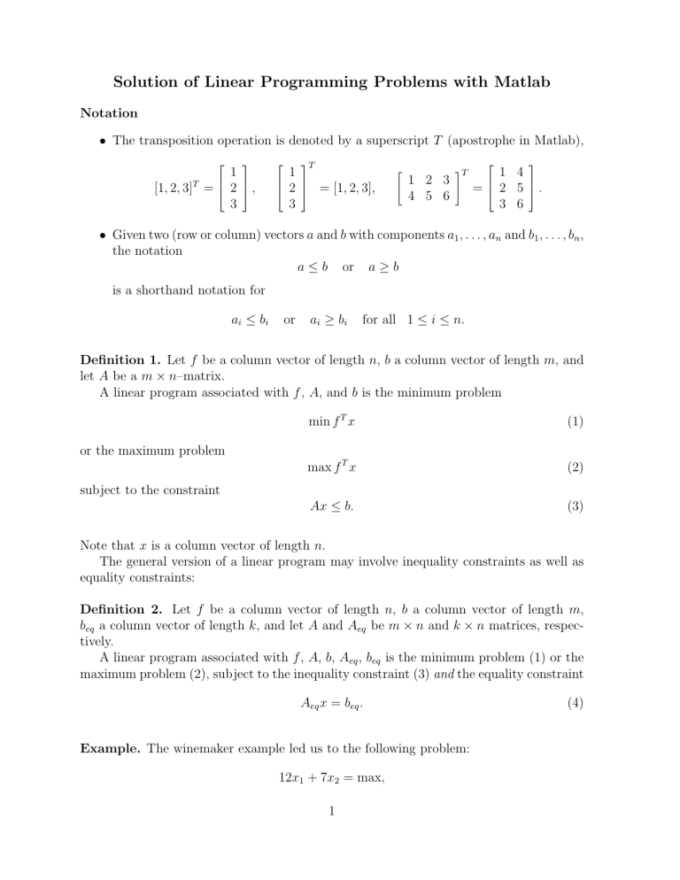
Solution of Linear Programming Problems with Matlab
Notation
• The transposition operation is denoted by a superscript T (apostrophe in Matlab),


1


T
[1, 2, 3] =  2  ,
3

T
1


 2  = [1, 2, 3],
3
"
1 2 3
4 5 6
#T


1 4


=  2 5 .
3 6
• Given two (row or column) vectors a and b with components a1 , . . . , an and b1 , . . . , bn ,
the notation
a ≤ b or a ≥ b
is a shorthand notation for
ai ≤ bi
or
ai ≥ bi
for all 1 ≤ i ≤ n.
Definition 1. Let f be a column vector of length n, b a column vector of length m, and
let A be a m × n–matrix.
A linear program associated with f , A, and b is the minimum problem
min f T x
(1)
max f T x
(2)
Ax ≤ b.
(3)
or the maximum problem
subject to the constraint
Note that x is a column vector of length n.
The general version of a linear program may involve inequality constraints as well as
equality constraints:
Definition 2. Let f be a column vector of length n, b a column vector of length m,
beq a column vector of length k, and let A and Aeq be m × n and k × n matrices, respectively.
A linear program associated with f , A, b, Aeq , beq is the minimum problem (1) or the
maximum problem (2), subject to the inequality constraint (3) and the equality constraint
Aeq x = beq .
Example. The winemaker example led us to the following problem:
12x1 + 7x2 = max,
1
(4)
subject to
2x1 + x2
3x1 + 2x2
x1
x2
If we define

"
f=
12
7
#
,



b=
≤
≤
≥
≥
10, 000
16, 000
0
0
10, 000
16, 000
0,
0.



,





A=
2
1
3
2
−1
0
0 −1



,

this problem can be identified with the linear programming maximum problem associated
with f , A, b. Likewise it can be identified with the linear programming minimum problem
associated with −f , A, b.
Solution of linear programming minimum problems with Matlab
Matlab provides the command linprog to find the minimizer (solution point) x of a linear
programming minimum problem. Without equality constraint the syntax is
x=linprog(f,A,b)
If you also want to retrieve the minimal value fmin = minx (f T x), type
[x,fmin]=linprog(f,A,b)
If inequality and equality constraint are given, use the commands
x=linprog(f,A,b,Aeq,beq)
or
[x,fmin]=linprog(f,A,b,Aeq,beq)
Let’s solve our winemaker problem:
>> f=[-12;-7];b=[10000;16000;0;0];A=[2 1;3 2;-1 0;0 -1];
>> [x,fopt]=linprog(f,A,b)
Optimization terminated successfully.
x =
1.0e+003 *
3.99999999989665
2
2.00000000013951
fopt =
-6.199999999973631e+004
This is the answer found in the class notes. The solution point is (4000, 2000), and the
maximum profit is $6, 2000.
Practice Problems
In each of the following problems first identify vectors and matrices such that the optimization problem can be written in the form of Definitions 1 or 2. Then use the linprog
command to solve the linear program.
Problem 1.
x1 + x2 = max
subject to
2x1 + x2
x1 + 2x2
x1
x2
≤
≤
≥
≥
29,
25,
2,
5.
Problem 2.
x1 + x2 + x3 + x4 + x5 = max
subject to
x1 + x2
x3 + x4
x2 + x3 + 2x4 + 5x5
xj
≤
≤
≤
≥
100,
70,
250,
0 (1 ≤ j ≤ 5).
Problem 3.
x1 + x2 + x3 + x4 + x5 = min
subject to
x1 + x2
x3 + x4
x2 + x3 + 2x4 + 5x5
xj
3
=
=
=
≥
100,
70,
250,
0 (1 ≤ j ≤ 5).