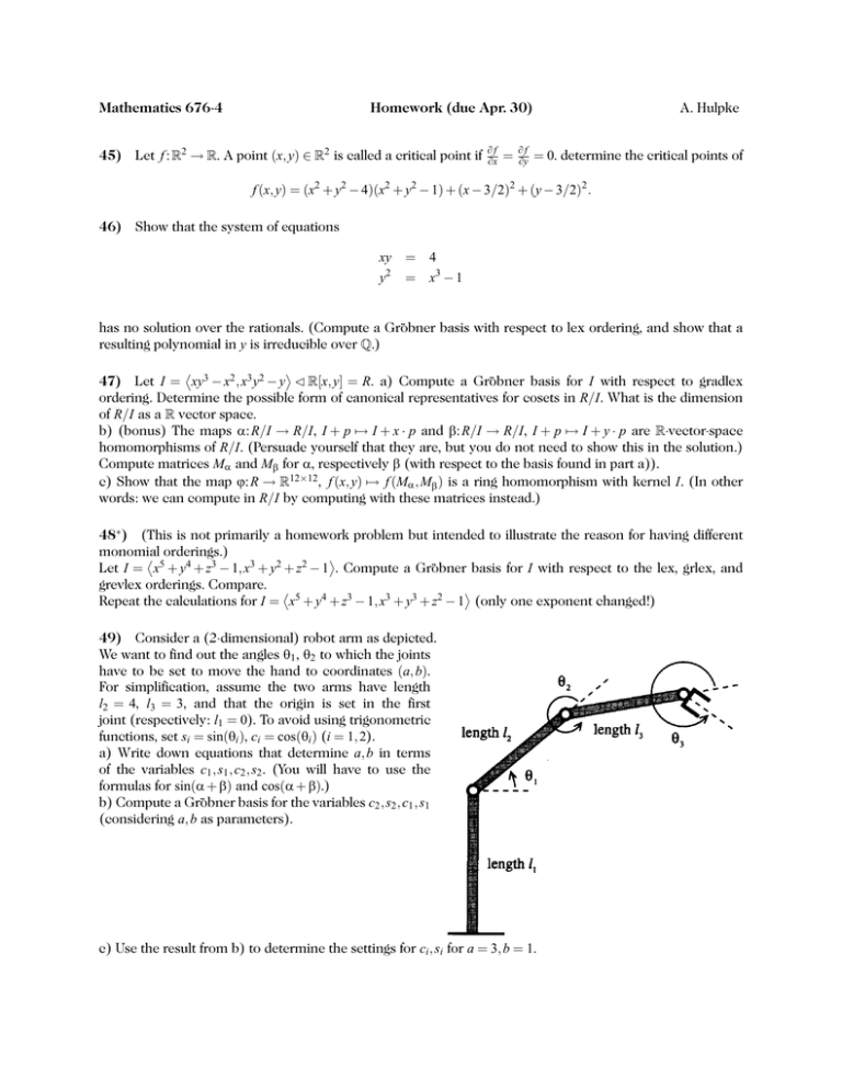
Mathematics 676-4
Homework (due Apr. 30)
45) Let f : R2 → R. A point (x, y) ∈ R2 is called a critical point if
∂f
∂x
=
∂f
∂y
A. Hulpke
= 0. determine the critical points of
f (x, y) = (x2 + y2 − 4)(x2 + y2 − 1) + (x − 3/2)2 + (y − 3/2)2 .
46) Show that the system of equations
xy = 4
y2 = x3 − 1
has no solution over the rationals. (Compute a Gröbner basis with respect to lex ordering, and show that a
resulting polynomial in y is irreducible over Q.)
47) Let I = xy3 − x2 , x3 y2 − y C R[x, y] = R. a) Compute a Gröbner basis for I with respect to gradlex
ordering. Determine the possible form of canonical representatives for cosets in R/I. What is the dimension
of R/I as a R vector space.
b) (bonus) The maps α: R/I → R/I, I + p 7→ I + x · p and β: R/I → R/I, I + p 7→ I + y · p are R-vector-space
homomorphisms of R/I. (Persuade yourself that they are, but you do not need to show this in the solution.)
Compute matrices Mα and Mβ for α, respectively β (with respect to the basis found in part a)).
c) Show that the map ϕ: R → R12×12 , f (x, y) 7→ f (Mα , Mβ ) is a ring homomorphism with kernel I. (In other
words: we can compute in R/I by computing with these matrices instead.)
48∗ ) (This is not primarily a homework problem but intended to illustrate the reason for having different
monomial
orderings.)
Let I = x5 + y4 + z3 − 1, x3 + y2 + z2 − 1 . Compute a Gröbner basis for I with respect to the lex, grlex, and
grevlex orderings. Compare. Repeat the calculations for I = x5 + y4 + z3 − 1, x3 + y3 + z2 − 1 (only one exponent changed!)
49) Consider a (2-dimensional) robot arm as depicted.
We want to find out the angles θ1 , θ2 to which the joints
have to be set to move the hand to coordinates (a, b).
For simplification, assume the two arms have length
l2 = 4, l3 = 3, and that the origin is set in the first
joint (respectively: l1 = 0). To avoid using trigonometric
functions, set si = sin(θi ), ci = cos(θi ) (i = 1, 2).
a) Write down equations that determine a, b in terms
of the variables c1 , s1 , c2 , s2 . (You will have to use the
formulas for sin(α + β) and cos(α + β).)
b) Compute a Gröbner basis for the variables c2 , s2 , c1 , s1
(considering a, b as parameters).
c) Use the result from b) to determine the settings for ci , si for a = 3, b = 1.
Gröbner bases in GAP On the course web page you find a file buchberg.g that provides a (not very
elaborate) implementation of Buchberger’s algorithm as well as some related functionality. You may use it for
all Gröbner basis calculations in the homework.
You can read this file in by putting it in the directory from which you start GAP and then call
gap> Read("buchberg.g");
To start using it, one has to define indeterminates and polynomials. Indeterminates are displayed either by
their internal numbers or you can prescribe names. (Note however that the names hide the internal numbers
and these numbers are basis for the monomial orderings. the best is to define a set of variables at the start
and then not to redefine them afterwards.
gap>
x_1
gap>
x
gap>
y
gap>
2
x:=X(Rationals,1); # number
x:=X(Rationals,"x");
y:=X(Rationals,"y");
IndeterminateNumberOfUnivariateLaurentPolynomial(y);
The three orders from the lecture are defined as MonomialLexOrder, MonomialGrlexOrder and MonomialGrevlexOrde
LeadingTerm gives the leading term of a polynomial.
gap> LeadingTerm(x*yˆ2+2*xˆ2*y,MonomialGrlexOrder);
2*xˆ2*y
GBasis computes a Gröbner basis. (You can set the info level as done here to get some information about
the calculations.)
gap> SetInfoLevel(InfoGrobner,1);
gap> B:=[x*y-yˆ2,yˆ2-x];
[ x*y-yˆ2, -x+yˆ2 ]
gap> G:=GBasis(B,MonomialGrlexOrder);
[ x*y-yˆ2, -x+yˆ2, x-xˆ2 ]
PolynomialReduction can be used to determine remainders. The first entry is the remainder, the second
the coefficients with respect to the list of basis elements. (Note that the division algorithm works slightly
different than the one in the book, thus if G is not a Gröbner basis you might get different remainders.)
gap> PolynomialReduction(xˆ5*y,G,MonomialGrlexOrder);
[ x, [ 1+y+yˆ2+yˆ3+xˆ4+xˆ3*y+xˆ2*yˆ2+x*yˆ3+yˆ4, 1+y+yˆ2+yˆ3+yˆ4, 0 ] ]
If you want to change the variable ordering, the best way is to permute the variables in the polynomials
instead (in the inverse order!). For example to change to an order y > x we could do:
gap> B2:=List(B,i->OnIndeterminates(i,(1,2)));
[ -xˆ2+x*y, -y+xˆ2 ]
gap> G:=GBasis(B2,MonomialGrlexOrder);
[ -xˆ2+x*y, -y+xˆ2, y-x*y, -y+yˆ2 ]
Problems marked with ∗ are bonus problems for extra credit.