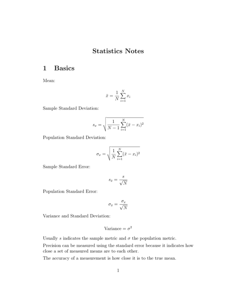
Statistics Notes
1
Basics
Mean:
x̄ =
N
1 X
xi
N i=1
Sample Standard Deviation:
sx =
v
u
u
t
N
1 X
(x̄ − xi )2
N − 1 i=1
Population Standard Deviation:
σx =
v
u
u
t
N
1 X
(x̄ − xi )2
N i=1
Sample Standard Error:
s
sx̄ = √
N
Population Standard Error:
σx
σx̄ = √
N
Variance and Standard Deviation:
Variance = σ 2
Usually s indicates the sample metric and σ the population metric.
Precision can be measured using the standard error because it indicates how
close a set of measured means are to each other.
The accuracy of a measurement is how close it is to the true mean.
1
2
Poor Man’s Error Propagation
Given the product equation:
z ± δz = (x ± δx)(y ± δy)
where x and y are subject to uncertainties, δx and δy, what is the uncertainly,
δz in z?
We can reexpress an uncertainty:
x ± δx
in the equivalent form:
δx
x 1±
x
!
Using this representation we can now express our product equation using:
δx
z ± δz = xy 1 ±
x
!
δy
1±
y
!
Multiplying out the terms in brackets and assuming that δxδy is negligible
(we’re assuming that the errors are very small), then
δx δy
+
z ± δz = xy 1 ±
x
y
That is
δp
z ± δz = 1 ±
p
where
p=
δx δy
+
x
y
2
!
!!
What this tells us is that the fractional error in z is given by the sum of the
fractional errors in x and y. For example, if the error in x is 2% and the
error in y is 3%, then the error in z is 5%.
3
Rule of Quadrature
The poor man’s approach to estimating errors overestimates the errors, instead an alternative approach known as the rule of quadrature is used which
gives more reasonable estimate for how errors propagate through equations.
Consider a quantity, Q which is to be calculated from several observed variables, a, b, c, . . .:
Q = f (a, b, c, . . .)
Suppose that a, b, c, . . . are measured N times. We can then calculate N
different values for Q. We can also calculate the mean and variance for the
set of measurements a, b, c, . . .:
σa2
N
1 X
(∆ai )2
=
N i=1
where ∆ai = ai − ā and also the variance of Q,
2
σQ
=
N
1 X
(∆Qi )2
N i=1
(1)
where Q̄ = f (ā, b̄, . . .), Qi = f (ai , bi , . . .) , and ∆Qi = Qi − Q̄. The ∆Qi can
be approximated by the following total derivative:
∂Q
∂Q
∆Qi ∼
∆ai +
∆bi + . . .
=
∂a
∂b
Inserting the above equation into equation (1) yields:
2
σQ
N
1 X
∂Q
∂Q
=
∆ai +
∆bi + . . .
N i=1 ∂a
∂b
3
!2
If the square term is expanded we get two types of term, one of which is the
cross term:
∂Q ∂Q
∆ai ∆bi
∂a ∂b
The cross terms, since they contain quantities that are equally likely to be
positive or negative, add up to near zero. Therefore we can drop the cross
terms to give:

N
1 X
∂Q
2

σQ
=
N i=1
∂a
!2
∂Q
(∆ai )2 +
∂b

!2
(∆bi )2 + . . .
This can be rewritten as
2
σQ
=
∂Q
∂a
2
σQ
!2
=
N
∂Q
1 X
∆a2i +
N i=1
∂b
∂Q
∂a
!2
σa2
∂Q
+
∂b
!2
N
1 X
∆b2 + . . .
N i=1 i
!2
σb2 + . . .
Normally we are more interested in the standard error than the standard
deviation. Given that the standard deviation is related to the standard error
by:
σ
2
σm̄
=√
N
√
2
so that σ = σm̄
N , then we can replace the √
standard deviations on both
sides with the standard errors (note that the N cancel on both sides) to
yield:
2
σQ̄
=
∂Q
∂a
!2
σā2
∂Q
+
∂b
or
4
!2
σb̄2 + . . .
σQ̄ =
v
u
u
t
∂Q
∂a
!2
∂Q
σā2 +
∂b
5
!2
σb̄2 + . . .
(2)