Artifical Intelligent
Mehdi Ebady Manaa
3rd class – Department of Network
College of IT- University of Babylon
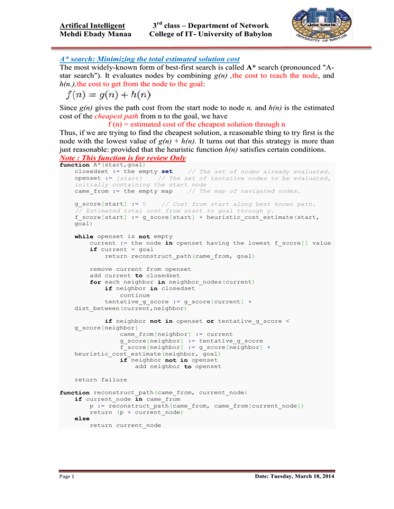
A* search: Minimizing the total estimated solution cost
The most widely-known form of best-first search is called A* search (pronounced "Astar search"). It evaluates nodes by combining g(n) ,the cost to reach the node, and
h(n.),the cost to get from the node to the goal:
Since g(n) gives the path cost from the start node to node n, and h(n) is the estimated
cost of the cheapest path from n to the goal, we have
f (n) = estimated cost of the cheapest solution through n
Thus, if we are trying to find the cheapest solution, a reasonable thing to try first is the
node with the lowest value of g(n) + h(n). It turns out that this strategy is more than
just reasonable: provided that the heuristic function h(n) satisfies certain conditions.
Note : This function is for review Only
function A*(start,goal)
closedset := the empty set
// The set of nodes already evaluated.
openset := {start}
// The set of tentative nodes to be evaluated,
initially containing the start node
came_from := the empty map
// The map of navigated nodes.
g_score[start] := 0
// Cost from start along best known path.
// Estimated total cost from start to goal through y.
f_score[start] := g_score[start] + heuristic_cost_estimate(start,
goal)
while openset is not empty
current := the node in openset having the lowest f_score[] value
if current = goal
return reconstruct_path(came_from, goal)
remove current from openset
add current to closedset
for each neighbor in neighbor_nodes(current)
if neighbor in closedset
continue
tentative_g_score := g_score[current] +
dist_between(current,neighbor)
if neighbor not in openset or tentative_g_score <
g_score[neighbor]
came_from[neighbor] := current
g_score[neighbor] := tentative_g_score
f_score[neighbor] := g_score[neighbor] +
heuristic_cost_estimate(neighbor, goal)
if neighbor not in openset
add neighbor to openset
return failure
function reconstruct_path(came_from, current_node)
if current_node in came_from
p := reconstruct_path(came_from, came_from[current_node])
return (p + current_node)
else
return current_node
Page 1
Date: Tuesday, March 18, 2014
Artifical Intelligent
Mehdi Ebady Manaa
3rd class – Department of Network
College of IT- University of Babylon
Comperhensive Example for Function A*
1) Add the starting square (or node) to the open list.
2) Repeat the following:
a) Look for the lowest F cost square on the open list. We refer to this as the current square.
b) Switch it to the closed list.
c) For each of the 8 squares adjacent to this current square …
 If it is not walkable or if it is on the closed list, ignore it. Otherwise do the
following.
 If it isn’t on the open list, add it to the open list. Make the current square the parent of this
square. Record the F, G, and H costs of the square.
 If it is on the open list already, check to see if this path to that square is better, using G
cost as the measure. A lower G cost means that this is a better path. If so, change the
parent of the square to the current square, and recalculate the G and F scores of the
square. If you are keeping your open list sorted by F score, you may need to resort the list
to account for the change.
d) Stop when you:
 Add the target square to the closed list, in which case the path has been found
 Fail to find the target square, and the open list is empty. In this case, there is no path.
3) Save the path. Working backwards from the target square, go from each square to its parent square
until you reach the starting square. That is your path.
(2)




Green = A (Start Point)
Red = B (Goal)
Blue= Obstacle Node
G cost, we will assign a cost of 10 to each
horizontal or vertical square moved, and a cost
of 14 for a diagonal move
 H Cost is the Manhattan Distance as an
example in vertical and horizontal only.
 Begin at the starting point A and add it to an “open list” of squares to
be considered.
 Look at all the reachable or walkable squares adjacent to the
starting point, ignoring squares with walls, water, or other illegal
terrain. Add them to the open list, too. For each of these squares,
save point A as its “parent square”.
 Drop the starting square A from your open list, and add it to a
“closed list” of squares that you don’t need to look at again for now.
(3)
The F score for each square,
again, is simply calculated by
adding G and H together.
Page 2
Date: Tuesday, March 18, 2014
Artifical Intelligent
Mehdi Ebady Manaa
3rd class – Department of Network
College of IT- University of Babylon
Continuing the Search
To continue the search, we simply choose the lowest F score square from all those that are
on the open list (here we have 8 open nodes). We then do the following with the selected
square:
4) Drop it from the open list and add it to the closed list.
5) Check all of the adjacent squares. Ignoring those that are on the closed list or
unwalkable (terrain with walls, water, or other illegal terrain), add squares to the open
list if they are not on the open list already. Make the selected square the “parent” of
the new squares.
6) If an adjacent square is already on the open list, check to see if this path to that square
is a better one. In other words, check to see if the G score for that square is lower if
we use the current square to get there. If not, don’t do anything.
On the other hand, if the G cost of the new path is lower, change the parent of the
adjacent square to the selected square (in the diagram above, change the direction of
the pointer to point at the selected square). Finally, recalculate both the F and G
scores of that square. If this seems confusing, you will see it illustrated below.
(5)
(4)
(6)
Page 3
Date: Tuesday, March 18, 2014
Artifical Intelligent
Mehdi Ebady Manaa
3rd class – Department of Network
College of IT- University of Babylon
(6)
(8)
A* Characteristics
1. A* search is both complete and optimal.
The optimality of A* is straightforward to analyze if it is used with TREESEARCH. In this case, A* is optimal if h(n) is an admissible heuristic-that is,
provided that h(n) never overestimates the cost to reach the goal. Admissible
heuristics (that is, it must not overestimate the distance to the goal) are by nature
optimistic, because they think the cost of solving the problem is less than it
actually is. Since g(n) is the exact cost to reach n, we have as immediate
consequence that f (n) never overestimates the true cost of a solution through n.
An obvious example of an admissible heuristic is the straight-line distance hSLD
that we used in getting to Bucharest example. Straight-line distance is admissible
because the shortest path between any two points is a straight line, so the straight
line cannot be an overestimate.
2. A* uses a best-first search and finds a least-cost path from a given initial node to
one goal node (out of one or more possible goals).
Page 4
Date: Tuesday, March 18, 2014
Artifical Intelligent
Mehdi Ebady Manaa
3rd class – Department of Network
College of IT- University of Babylon
3. As A* traverses the graph, it follows a path of the lowest expected total cost or
distance, keeping a sorted priority queue of alternate path segments along the way.
4. It uses a knowledge-plus-heuristic cost function of node x (usually denoted f(x)) to
determine the order in which the search visits nodes in the tree. The cost function is
a sum of two functions:
 the past path-cost function, which is the known distance from the starting node
to the current node x (usually denoted g(x))
 a future path-cost function, which is an admissible "heuristic estimate" of the
distance from x to the goal (usually denoted h(x)).
Example
An example of an A star (A*) algorithm in action where nodes are cities connected
with roads and h(x) is the straight-line distance to target point:
Example
Illustration of A* search for finding path from a start node to a goal node in a
robot motion planning problem. The empty circles represent the nodes in the open set,
i.e., those that remain to be explored, and the filled ones are in the closed set. Color on
each closed node indicates the distance from the start: the greener, the farther. One
can first see the A* moving in a straight line in the direction of the goal, then when
hitting the obstacle, it explores alternative routes through the nodes from the open set.
Page 5
Date: Tuesday, March 18, 2014