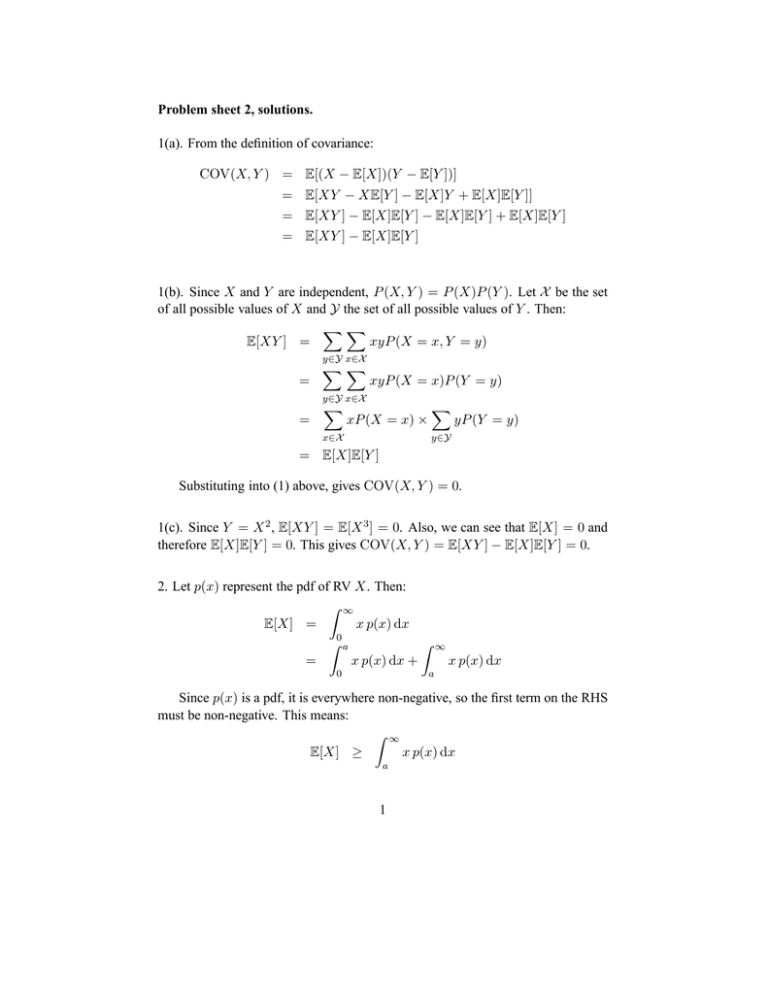
Problem sheet 2, solutions.
1(a). From the definition of covariance:
COV(X, Y ) = E[(X − E[X])(Y − E[Y ])]
= E[XY − XE[Y ] − E[X]Y + E[X]E[Y ]]
= E[XY ] − E[X]E[Y ] − E[X]E[Y ] + E[X]E[Y ]
= E[XY ] − E[X]E[Y ]
1(b). Since X and Y are independent, P (X, Y ) = P (X)P (Y ). Let X be the set
of all possible values of X and Y the set of all possible values of Y . Then:
XX
E[XY ] =
xyP (X = x, Y = y)
y∈Y x∈X
=
XX
xyP (X = x)P (Y = y)
y∈Y x∈X
=
X
X
xP (X = x) ×
x∈X
yP (Y = y)
y∈Y
= E[X]E[Y ]
Substituting into (1) above, gives COV(X, Y ) = 0.
1(c). Since Y = X 2 , E[XY ] = E[X 3 ] = 0. Also, we can see that E[X] = 0 and
therefore E[X]E[Y ] = 0. This gives COV(X, Y ) = E[XY ] − E[X]E[Y ] = 0.
2. Let p(x) represent the pdf of RV X. Then:
Z ∞
E[X] =
x p(x) dx
Z
Z0 a
x p(x) dx +
=
∞
x p(x) dx
a
0
Since p(x) is a pdf, it is everywhere non-negative, so the first term on the RHS
must be non-negative. This means:
Z ∞
x p(x) dx
E[X] ≥
a
1
Since a is the lower bound on the integral above, we can write
Z ∞
Z ∞
a p(x) dx
x p(x) dx ≥
a
a
which gives
E[X] ≥
∞
Z
a p(x) dx
a
= a
Z
∞
p(x) dx
a
= a P (X ≥ a)
from which the required result follows.
3. First, note that
P (|X − µX | ≥ a) = P ((X − µX )2 ≥ a2 )
Here, (X − µX )2 is a non-negative RV. Using the Markov inequality, we get:
P ((X − µX )2 ≥ a2 ) ≤
=
E[(X − µX )2 ]
a2
2
σX
a2
as required.
4. If θ̂n is unbiased, we can write
P (|θ̂n − θ| ≥ ) = P (|θ̂n − E[θ̂n ]| ≥ )
Applying the Chebyshev inequality to the RHS, we get:
P (|θ̂n − E[θ̂n ]| ≥ ) ≤
VAR(θ̂n )
2
From the RHS above we can see that if
lim VAR(θ̂n ) = 0
n→∞
the estimator converges in probability to θ, that is, it is consistent.
2
5. Let X̄n denote the sample mean derived from n observations. This is easily
shown to be unbiased. Using the Chebyshev inequality:
P (|X̄n − µX | ≥ ) ≤
VAR(X̄n )
2
But:
VAR(X̄n ) = VAR
=
1
(X1 + . . . + Xn )
n
2
σX
n
Therefore
2
σX
n2
P (|X̄n − µX | ≥ ) ≤
and
lim P (|X̄n − µX | ≥ ) = 0
n→∞
which means X̄n converges in probability to the true mean µX , as required.
6(a). Log-likelihood:
n
L(µ, Σ) = −
n
1X
dn
(Xi − µ)T Σ−1 (Xi − µ)
log(2π) − log(|Σ|) −
2
2
2
i=1
6(b). We proceed in two steps: we first treat Σ as fixed, and maximize L to get
a value µ̂(Σ) which maximizes L for a given matrix parameter Σ. Taking the
derivative of the L wrt vector µ, we get:
n
X
d
(Xi − µ))T
L = (Σ−1
dµ
i=1
Setting the derivative to zero, taking the transpose of both sides and pre-multiplying
by Σ, we get:
0 =
n
X
(Xi − µ)
i=1
3
Solving for µ:
n
1X
Xi
n
µ̂(Σ) =
i=1
= X̄
Since this solution does not depend on Σ, X̄ is the maximum likelihood estimator of µ for any Σ. To obtain Σ̂ we plug µ̂(Σ) = X̄ into the log-likelihood to
obtain
n
n
1X
dn
(Xi − X̄)T Σ−1 (Xi − X̄)
log(2π) − log(|Σ|) −
−
2
2
2
(1)
i=1
and maximize this function wrt Σ.
We first introduce a sample covariance matrix S defined as follows:
n
S =
1X
(Xi − X̄)(Xi − X̄)T
n
i=1
This allows us to re-write the quadratic form in (1) as a matrix trace:
n
X
(Xi − X̄)T Σ−1 (Xi − X̄) = n Tr(Σ−1 S)
i=1
where Tr(·) denotes the trace of its matrix argument.
This in turn allows us to write the derivative of (1) wrt Σ as follows:
−
n d
n d
log(|Σ|) −
Tr(Σ−1 S)
2 dΣ
2 dΣ
At this point we make use of two useful matrix derivatives (these can be found
in Appendix C of Bishop and the note “Matrix Identities” by Roweis, available on
the course website):
∂
log(|A|) = (A−1 )T
∂A
∂
Tr(X−1 A) = −X−1 AT X−1
∂X
This gives the derivative (2) in the following form (where we make use of the
fact that both Σ−1 and S are symmetric):
n
n
− Σ−1 + Σ−1 SΣ−1
2
2
4
Setting to zero and solving, we get:
Σ̂ = S
n
1X
=
(Xi − X̄)(Xi − X̄)T
n
i=1
5