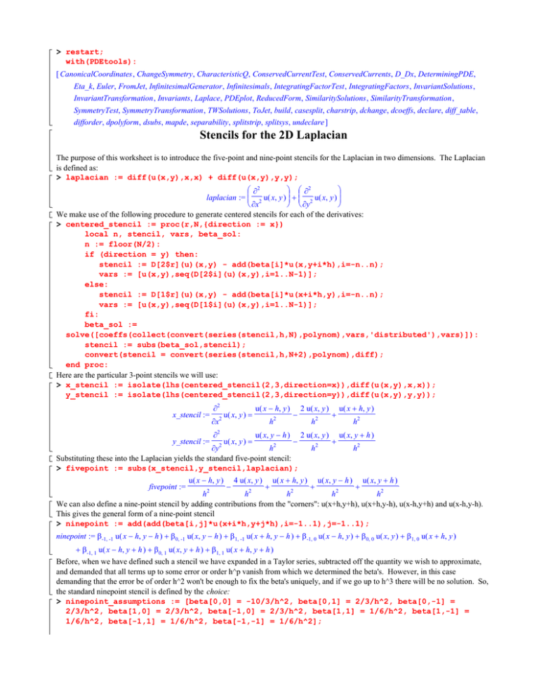
> restart;
with(PDEtools):
[ CanonicalCoordinates , ChangeSymmetry, CharacteristicQ, ConservedCurrentTest, ConservedCurrents, D_Dx, DeterminingPDE,
Eta_k, Euler, FromJet, InfinitesimalGenerator , Infinitesimals , IntegratingFactorTest , IntegratingFactors , InvariantSolutions ,
InvariantTransformation , Invariants , Laplace, PDEplot, ReducedForm, SimilaritySolutions , SimilarityTransformation ,
SymmetryTest, SymmetryTransformation , TWSolutions , ToJet, build, casesplit, charstrip, dchange , dcoeffs, declare, diff_table ,
difforder, dpolyform, dsubs, mapde, separability , splitstrip, splitsys, undeclare ]
Stencils for the 2D Laplacian
The purpose of this worksheet is to introduce the five-point and nine-point stencils for the Laplacian in two dimensions. The Laplacian
is defined as:
> laplacian := diff(u(x,y),x,x) + diff(u(x,y),y,y);
 ∂2
  ∂2

laplacian :=  2 u( x, y )  +  2 u( x, y ) 
 ∂x
  ∂y

We make use of the following procedure to generate centered stencils for each of the derivatives:
> centered_stencil := proc(r,N,{direction := x})
local n, stencil, vars, beta_sol:
n := floor(N/2):
if (direction = y) then:
stencil := D[2$r](u)(x,y) - add(beta[i]*u(x,y+i*h),i=-n..n);
vars := [u(x,y),seq(D[2$i](u)(x,y),i=1..N-1)];
else:
stencil := D[1$r](u)(x,y) - add(beta[i]*u(x+i*h,y),i=-n..n);
vars := [u(x,y),seq(D[1$i](u)(x,y),i=1..N-1)];
fi:
beta_sol :=
solve([coeffs(collect(convert(series(stencil,h,N),polynom),vars,'distributed'),vars)]):
stencil := subs(beta_sol,stencil);
convert(stencil = convert(series(stencil,h,N+2),polynom),diff);
end proc:
Here are the particular 3-point stencils we will use:
> x_stencil := isolate(lhs(centered_stencil(2,3,direction=x)),diff(u(x,y),x,x));
y_stencil := isolate(lhs(centered_stencil(2,3,direction=y)),diff(u(x,y),y,y));
x_stencil :=
y_stencil :=
∂2
2
∂x
∂2
2
u( x, y ) =
u( x, y ) =
u( x − h, y )
h
2
u( x, y − h )
2
−
−
∂y
h
Substituting these into the Laplacian yields the standard five-point stencil:
> fivepoint := subs(x_stencil,y_stencil,laplacian);
2 u( x, y )
h
2
2 u( x, y )
h
2
+
+
u( x + h, y )
h2
u( x, y + h )
h2
4 u( x, y ) u( x + h, y ) u( x, y − h ) u( x, y + h )
−
+
+
+
h2
h2
h2
h2
h2
We can also define a nine-point stencil by adding contributions from the "corners": u(x+h,y+h), u(x+h,y-h), u(x-h,y+h) and u(x-h,y-h).
This gives the general form of a nine-point stencil
> ninepoint := add(add(beta[i,j]*u(x+i*h,y+j*h),i=-1..1),j=-1..1);
fivepoint :=
u( x − h, y )
ninepoint := β-1, -1 u( x − h, y − h ) + β0, -1 u( x, y − h ) + β1, -1 u( x + h, y − h ) + β-1, 0 u( x − h, y ) + β0, 0 u( x, y ) + β1, 0 u( x + h, y )
+ β-1, 1 u( x − h, y + h ) + β0, 1 u( x, y + h ) + β1, 1 u( x + h, y + h )
Before, when we have defined such a stencil we have expanded in a Taylor series, subtracted off the quantity we wish to approximate,
and demanded that all terms up to some error or order h^p vanish from which we determined the beta's. However, in this case
demanding that the error be of order h^2 won't be enough to fix the beta's uniquely, and if we go up to h^3 there will be no solution. So,
the standard ninepoint stencil is defined by the choice:
> ninepoint_assumptions := [beta[0,0] = -10/3/h^2, beta[0,1] = 2/3/h^2, beta[0,-1] =
2/3/h^2, beta[1,0] = 2/3/h^2, beta[-1,0] = 2/3/h^2, beta[1,1] = 1/6/h^2, beta[1,-1] =
1/6/h^2, beta[-1,1] = 1/6/h^2, beta[-1,-1] = 1/6/h^2];
ninepoint := subs(ninepoint_assumptions,ninepoint);
ninepoint_assumptions :=

10
2
2
2
2
1
1
1
1 
 β0, 0 = −

, β 0, 1 =
, β0, -1 =
, β 1, 0 =
, β-1, 0 =
, β 1, 1 =
, β1, -1 =
, β-1, 1 =
, β-1, -1 =
2
2
2
2
2
2
2
2

3h
3h
3h
3h
3h
6h
6h
6h
6 h2 
ninepoint :=
+
1 u( x − h, y − h )
6
h
2
1 u( x − h, y + h )
2
+
+
2 u( x, y − h )
3
h
2
2 u( x, y + h )
2
+
1 u( x + h, y − h )
+
6
h
2
+
2 u( x − h, y )
3
h
2
10 u( x, y )
−
3
h
2
+
2 u( x + h, y )
h2
3
1 u( x + h, y + h )
6
3
6
h
h
h2
We can calculate the error in the two stencil in the standard way:
> fivepoint_error := convert(series(laplacian-fivepoint,h),diff);
ninepoint_error := convert(series(laplacian-ninepoint,h),diff);
 1  ∂4
 1  ∂4


fivepoint_error :=  −  4 u( x, y )  −
u( x, y )   h2 + O( h4 )

4
 12  ∂y
 12  ∂x

 1  ∂4
 1  ∂4
 1  ∂4
 2
4


ninepoint_error :=  −  4 u( x, y )  −  2 2 u( x, y )  −
 4 u( x, y )   h + O( h )
12
6
12

 ∂x

 ∂y ∂ x

 ∂y

Notice that they are both errors of order h^2. But the error of the ninepoint stencil has a very interesting form. Let's calculate the
Laplacian of the Laplacian of u:
> laplacianoflaplacian := Laplacian^2 = expand(subs(u(x,y)=laplacian,laplacian));
 ∂4

 ∂4
  ∂4

laplacianoflaplacian := Laplacian 2 =  4 u( x, y )  + 2  2 2 u( x, y )  +  4 u( x, y ) 
 ∂x

 ∂y ∂ x
  ∂y

But this is just proportional to the h^2 constribution to the ninepoint error; i.e.,
> ninepoint_error :=
subs(isolate(laplacianoflaplacian,diff(u(x,y),x,x,x,x)),ninepoint_error);
Laplacian 2
h2 + O( h4 )
12
Hence, if the Laplacian of u is itself zero, then the h^2 part of the ninepoint error vanishes and we have a much more accurate stencil.
This indeed occurs when we are solve Laplace's equation, which is
> laplace_eq := laplacian = 0;
possion_eq := laplacian - f(x,y) = 0;
ninepoint_error := −
 ∂2
  ∂2

laplace_eq :=  2 u( x, y )  +  2 u( x, y )  = 0
 ∂x
  ∂y

 ∂2
  ∂2

possion_eq :=  2 u( x, y )  +  2 u( x, y )  − f( x, y ) = 0

 ∂x
  ∂y
We will also be interested in the solution to the Poisson equation, which is also given above. In this, f is supposed to be a known
function. We can use either the fivepoint or ninepoint stencils in each of these equations:
> laplace_stencil_5 := fivepoint = 0;
laplace_stencil_9 := ninepoint = 0;
possion_stencil_5 := fivepoint - f(x,y) = 0;
possion_stencil_9 := ninepoint - f(x,y) = 0;
laplace_stencil_5 :=
laplace_stencil_9 :=
+
1 u( x − h, y − h )
6
1 u( x − h, y + h )
6
h
2
h
+
2
3
h
2
1 u( x − h, y − h )
6
h
2
h2
2 u( x, y − h )
3
2 u( x, y + h )
possion_stencil_5 :=
possion_stencil_9 :=
+
u( x − h, y )
+
h
2
2
−
6
h
h
2
h
+
u( x + h, y )
h2
2
2
+
u( x + h, y )
h
2
1 u( x + h, y − h )
6
+
+
u( x, y − h )
h2
2 u( x − h, y )
3
h
2
−
+
u( x, y + h )
h2
10 u( x, y )
3
h
2
+
=0
2 u( x + h, y )
3
h2
=0
4 u( x, y )
2 u( x, y − h )
+
1 u( x + h, y − h )
h2
6
h
3
+
h2
1 u( x + h, y + h )
u( x − h, y )
+
4 u( x, y )
−
h
2
+
+
u( x, y − h )
h
2
2 u( x − h, y )
3
h
2
+
−
u( x, y + h )
h2
10 u( x, y )
3
h
2
+
− f( x, y ) = 0
2 u( x + h, y )
3
h2
+
1 u( x − h, y + h )
+
2 u( x, y + h )
2
+
1 u( x + h, y + h )
− f( x, y ) = 0
6
3
6
h
h
h2
As usual, the error in a given stencil is calculated by expanding about h = 0 and substituting in the original PDE. We get
> err_laplace_stencil_5 :=
convert(dsubs(isolate(laplace_eq,diff(u(x,y),x,x)),simplify(convert(series(lhs(laplace_st
encil_5),h=0,4),diff))),D);
err_laplace_stencil_9 :=
convert(dsubs(isolate(laplace_eq,diff(u(x,y),x,x)),simplify(convert(series(lhs(laplace_st
encil_9),h=0,10),diff))),D);
err_poisson_stencil_5 :=
convert(dsubs(isolate(possion_eq,diff(u(x,y),x,x)),simplify(convert(series(lhs(possion_st
encil_5),h=0,4),diff))),D);
err_poisson_stencil_9 :=
convert(dsubs(isolate(possion_eq,diff(u(x,y),x,x)),simplify(convert(series(lhs(possion_st
encil_9),h=0,6),diff))),D);
2
1
err_laplace_stencil_5 :=
err_laplace_stencil_9 :=
6
1
3024
D2, 2, 2, 2( u )( x, y ) h2 + O( h4 )
D2, 2, 2, 2, 2, 2, 2, 2( u )( x, y ) h6 + O( h8 )
1
1
1

D2, 2( f )( x, y ) +
D1, 1( f )( x, y )  h2 + O( h4 )
err_poisson_stencil_5 :=  D2, 2, 2, 2( u )( x, y ) −
12
12
6

err_poisson_stencil_9 :=
1
1

 1
1
1

 D2, 2( f )( x, y ) +
D1, 1( f )( x, y )  h2 + 
D2, 2, 2, 2( f )( x, y ) +
D1, 1, 2, 2( f )( x, y ) +
D1, 1, 1, 1( f )( x, y )  h4 + O( h6 )
 12
12

 360
90
360

As we expected, the error for the ninepoint stencil on the Laplace equation is much more accurate than for the fivepoint stencil. The
error terms for the Poisson equation are interesting, They both appear to be of order h^2, but the lowest order error terms in the
ninepoint version are expressed entirely in terms of the known function f. In other words, we can calculate them explicitly. This
suggests we modify the original ninepoint stencil for the Poisson equation as follows:
> possion_stencil_9_modified := ninepoint - f(x,y) - convert(err_poisson_stencil_9,polynom)
= 0;
possion_stencil_9_modified :=
+
1 u( x − h, y + h )
h2
6
+
1 u( x − h, y − h )
6
h
2
2 u( x, y + h )
3
h2
+
+
2 u( x, y − h )
3
h
2
1 u( x + h, y + h )
6
h2
+
1 u( x + h, y − h )
6
h
2
+
2 u( x − h, y )
3
h
2
−
10 u( x, y )
3
h
2
+
2 u( x + h, y )
3
h2
1
1

D ( f )( x, y )  h2
− f( x, y ) −  D2, 2( f )( x, y ) +
12 1, 1
 12

1
1
 1

D
( f )( x, y ) +
D
( f )( x, y ) +
D
( f )( x, y )  h4 = 0
− 
 360 2, 2, 2, 2
90 1, 1, 2, 2
360 1, 1, 1, 1

The error in this modified Poisson stencil is now h^6, just like for the ninepoint Laplace equation stencil.
> err_poisson_stencil_9_modified :=
convert(dsubs(isolate(possion_eq,diff(u(x,y),x,x)),simplify(convert(series(lhs(possion_st
encil_9_modified),h=0,10),diff))),D);
 1
17
1
err_poisson_stencil_9_modified := 
D2, 2, 2, 2, 2, 2, 2, 2( u )( x, y ) −
D2, 2, 2, 2, 2, 2( f )( x, y ) +
D
( f )( x, y )
 3024
60480
1344 1, 1, 2, 2, 2, 2
+
>
5
12096
D1, 1, 1, 1, 2, 2( f )( x, y ) +
1
20160

D1, 1, 1, 1, 1, 1( f )( x, y )  h6 + O( h8 )
