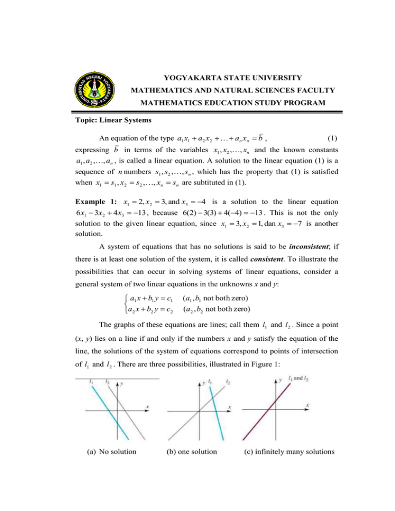
YOGYAKARTA STATE UNIVERSITY
MATHEMATICS AND NATURAL SCIENCES FACULTY
MATHEMATICS EDUCATION STUDY PROGRAM
Topic: Linear Systems
An equation of the type a1 x1  a2 x2    an xn  b ,
(1)
expressing b in terms of the variables x1 , x2 ,, xn and the known constants
a1 , a2 ,, an , is called a linear equation. A solution to the linear equation (1) is a
sequence of n numbers s1 , s 2 ,, s n , which has the property that (1) is satisfied
when x1  s1 , x2  s2 ,, xn  sn are subtituted in (1).
Example 1: x1  2, x2  3, and x3  4 is a solution to the linear equation
6 x1  3x2  4 x3  13 , because 6(2)  3(3)  4(4)  13 . This is not the only
solution to the given linear equation, since x1  3, x2  1, dan x3  7 is another
solution.
A system of equations that has no solutions is said to be inconsistent; if
there is at least one solution of the system, it is called consistent. To illustrate the
possibilities that can occur in solving systems of linear equations, consider a
general system of two linear equations in the unknowns x and y:
 a1 x  b1 y  c1

a 2 x  b2 y  c2
(a1 , b1 not both zero)
(a 2 , b2 not both zero)
The graphs of these equations are lines; call them l1 and l 2 . Since a point
(x, y) lies on a line if and only if the numbers x and y satisfy the equation of the
line, the solutions of the system of equations correspond to points of intersection
of l1 and l 2 . There are three possibilities, illustrated in Figure 1:
(a) No solution
(b) one solution
(c) infinitely many solutions
The lines l1 and l 2 may be parallel, in which case there is no intersection
and consequently no solution to the system. The lines l1 and l 2 may intersect at
only one point, in which case the system has exactly one solution. The lines l1
and l 2 may coincide, in which case there are infinitely many points of intersection
and consequently infinitely many solutions to the system.
Although we have considered only two equations with two unknowns here, we
will show later that the same three possibilities hold for arbitrary linear systems
Every system of linear equations has no solutions, or has exactly one solution, or
has infinitely many solutions.
More generally, a linear system is a system of m linear equations in n
unknowns, and can be conveniently denoted by
 a11 x1  a12 x 2    a1n x n  b1
 a x  a x  a x  b
 21 1
22 2
2n n
2






 a m1 x1  a m 2 x 2    a mn x n  bm .
(2)
A solution to a linear system (2) is a sequence of n numbers s1 , s 2 ,, s n , which
has the property that each equation in (2) is satisfied when
x1  s1 , x2  s2 ,, xn  sn are subtituted in (2).
The Solution of The Linear System
The basic method for solving a system of linear equations is to replace the
given system by a new system that has the same solution set but is easier to solve.
This new system is generally obtained in a series of steps by applying the
following three types of operations to eliminate unknowns systematically:
The Linear Equation Operation
1. Interchange two equations.
2. Multiply an equation by a nonzero constant.
3. Add a multiple of one equation to another.
Example 2: Given the linear system:
 x  y  2z  9

2 x  4 y  3 z  1
3x  6 y  5 z  0

To eliminate x from the second equation, we add (  2 ) times the first equation to
the second one to obtain
9
 x  y  2z 

4 y  3z   17

3x  6 y  5 z 
0

To eliminate x from the second equation, we add (  3 ) times the first equation to
the third one to obtain
9
x  y  2z 

2 y  7 z   17


3 y  11z   27

Multiply the second equation with 1 2 , to obtain
9
x  y  2z 

y  72 z   172


3 y  11z   27

Added (  3 ) times the second equation to the third one to obtain
9
x  y  2z 

y  72 z   172


 12 z   32

Multiply the third equation with  2 , to obtain
x 




y
y
2z 
9
7
z   172
2
z
3
Added (  1) times the second equation to the first one to obtain
x 

 y


11
2
7
2
z
z 
z
35
2
17
2
3
Added (  112 ) times the third equation to the first one and ( 72 ) times the third
equation to the second one to obtain
 1
x

 y  2

z 3

We conclude that the solution of the linear system is x  1, y  2, z  3 .
Exercises 1:
1.
Which of the following are linear equations in x1 , x2 and x3 ?
(a) x1  5x2  2 x3  1
(b) x1  3x2  x1 x3  2
(c) x1  7 x2  3x3
2
(d) x1  x2  8x3  5
(e) x1
3
5
 2 x 2  x3  4
1
1
(f) x1  2 x2  x3  7 3
3
2.
Find the solution set of each of the following linear equations.
(a) 7 x  5 y  3 .
(b) 3x1  5x2  4 x3  7
(c)  8x1  2 x2  5x3  6 x4  1
(d) 3v  8w  2 x  y  4 z  0 .
3.
Find the solution of given the linear system.
 x  2y  z  8

(a)  x  3 y  2 z  1
 3x  4 y  7 z  10

4.
 2z  1
 2x

y  4z  7
(b)  3x 
6 x  2 y
z 0

(a) Find a linear equation in the variables x and y that has the general solution
x  5  2t , y  t .
(b) Show that x  t , y 
1
5
t  is also the general solution of the equation in
2
2
part (a).
5.
Consider the system of equations
 x

 x
2 x 

y  2z  a

z b
y  3z 
c
Show that for this system to be consistent, the constant a, b, and c must
satisfy c = a + b.
6.
Show that if the linear equations x1  kx2  c and x1  lx 2  d have the same
solution set, then the equations are identical.
7.
For which value(s) of the constant k does the system
 x y 3

2 x  2 y  k
have no solutions? Exactly one solution? Infinitely many solutions? Explain
your reasoning.
8.
Consider the system of equations
 ax  by  k

 cx  dy  l
ex  fy  m

Indicate what we can say about the relative positions of the lines ax  by  k ,
cx  dy  l , and ex  fy  m when
(a) the system has no solutions.
(b) the system has exactly one solution.
(c) the system has infinitely many solutions.
9.
If the system of equations in Exercise 8 is consistent, explain why at least one
equation can be discarded from the system without altering the solution set.
10. If k = l = m = 0 in Exercise 8, explain why the system must be consistent.
What can be said about the point of intersection of the three lines if the
system has exactly one solution?
YOGYAKARTA STATE UNIVERSITY
MATHEMATICS AND NATURAL SCIENCES FACULTY
MATHEMATICS EDUCATION STUDY PROGRAM
Topic: Matrices
Definition 1. An m n matrix A is a rectangular of mn real (or complex)
numbers arranged in m horizontal rows and n vertical columns :
 a11 a12
a
a
A   21 22
 


a m1 a m 2
The ith row of A, ai1 ai 2
 a1n 
 a 2 n 
.
  

 a mn 
(3)
 a1 j 
a 
2j
 ain  , (1  i  m); the jth column of A,   ,
  
 
 a mj 
(1 j n).
If m = n, we say that A is a square matrix of order n, and that the numbers
a11 , a22 , , ann form the main diagonal A. We refer to the number a ij , which is in
the ith row and jth column of A, and (3) often write as A  [aij ] . Sum of all main
diagonal is called trace A (tr A).
 1 2 3
Example 3: A  
 is an 2  3 matrix with
 1 0 1
1 4 
a12  2, a13  3, a22  0, a23  1. B  
 is an 2  2 matrix, with
2  3
1
tr ( A)  1  (3)  (2). C   1 is an 3 1 matrix or column matrix.
 2 
1 1 0 
D  2 0 1 is an 3 3 matrix, with tr ( A)  3 . E  3 is an 1 1 matrix.
3  1 2
F   1 0 2 is an 1 3 matrix or row matrix.
The Equality of Two Matrices
Definition 2. Two m n matrices A  [aij ] and B  [bij ] are said to be equal if
aij  bij , 1  i  m, 1  j  n , that is, if corresponding elements are equal.
Example 4: The matrices
1 2  1
 1 2 w
A  2  3 4  and B   2 x 4  are equal if w  1, x  3, y  0 and
0  4 5 
 y  4 z 
z  5.
Matrix Addition
Definition 3. If A = [aij] and B = [bij] are m n matrices, then A+B is a m n
matrix C =[cij], defined by cij = aij + bij ( 1  i  m,1  j  n ) and the difference
between A and B is D = [dij] noted as A  (1) B  A  B , defined by
d ij  aij  bij .
Example 5:
1.
1  2 4 
0 2  4
Given A  
and B  

.
 2  1 3
1 3 1 
1  0  2  2 4  (4) 1 0 0
Then A  B  

.
2  1  1  3 3  1  3 2 4
2.
2 3  5
2  1 3 
If A  
and B  

 , then
4 2 1 
 3 5  2
2  2 3  1  5  3 0 4  8
A B  

.
 4  3 2  5 1  2  1  3 3 
3.
4 8
 6  2
 10 4
Given A  
, B
and C  

 . Then

2 14
 21  3
10 4
8 - 2 - 4 20 2
 4  6  10
A  B  C

.
2  10 - 21 14  4  3 - 9 21
Additon Matrix Properties
Given A, B, C, and D are m n matrices.
(a) A + B = B + A.
(b) A + (B + C) = (A + B) + C.
(c) A + O = A. O matrix is called zero matrix or the addition identity.
(d) A + D = O. D   A is called the inverse addition matrix or the negative of
A.
Example 6:
4  1
0 0
and O  
1. Given A  

. Then
3
2
0 0
4  0  1  0 4  1
AO  

 = A.
2  0 3  0 2 3
 2 3 4
  2  3  4
. Then  A  
2. Given A  

, and we obtained
  4 5  2
 4  5 2
A  ( A)  O .
Scalar Multiplication
Definition 4. If A=[aij] is m n matrix and r is a real number, then scalar multiple
of A by r, rA, is the m n matrix B=[bij], where bij = raij ( 1  i  m,1  j  n ).
Example 7:
1.
4  2 3 
If r  3 and A  2  5 0  , then
3 6  2
4  2 3  (3)(4) (3)(2) (3)(3)   12 6  9
rA  32  5 0   (3)(2) (3)(5) (3)(0)     6 15 0 .
3 6  2  (3)(3) (3)(6) (3)(2)   9  18 6 
2.
 1 2
4 3
 1  3
, B
, and C  
Given A  


 . Then
3 4
2 1
 2  4
 1  12  5 2  9  15  6  22
A  3B  5C  

.
3  6  10 4  3  20  7  19
3.
 a b 
a b 
, B
Given A  

, and any scalar k . Then
  b 2a 
 b 2a 
 3ka 3kb 2ka 2kb  5ka kb
 5a b
3kA  2kB  


 k



.
 3kb 6ka 2kb 4ka  5kb 2ka
  5b 2a 
Scalar Multiplication Matrix Properties
If r and s are real number and A and B are matrices, then
(a) r(sA) = (rs)A.
(c) r(A + B) = rA + rB.
(b) (r + s)A = rA + sA.
(d) A(rB) = r(AB) = (rA)B.
2 - 1
 1 2 3
, and B   1 4. Then
Example 8: Given r  2 , A  

 2 0 1
0 - 2
2
 4
 1 2 3 
  8  2
A(rB)  
 2  8  
, and


8
0
 2 0 1  0

4

 4 1  8  2
r ( AB )  (-2)
.

0
- 4 0   8
Matrix Multiplication
Definition 5. If A = [aij] is an m  p matrix and B = [bij] is an p  n matrix, then
the product of A and B, denoted AB, is the m n matrix C = [cij], defined by
p
cij  ai1b1 j  ai 2 b2 j  ...  aip b pj   aik bkj (1  i  m, 1  j  n).
k 1
Example 9:
1.
- 2 5
 1 2  1
and B   4 - 3. Then
Given A  

3 1 4
 2 1
(1)(2)  (2)(4)  (1)(2) (1)(5)  (2)(3)  (1)(1) 4  2
AB  

.
 (3)(2)  (1)(4)  (4)(2) (3)(5)  (1)(3)  (4)(1) 6 16
2.
3
1  2
 1 4


2
1 and B   3 - 1. If AB=C then the (3,2) entry of
Given A  4
0
- 2 2
1  2
AB
is
c32,
which
is
R3(A)
x
C2(B).
We
now
have
 4
R3 ( A)  C 2 ( B)  0 1  2   1  5.
 2
3.
2
 1 x 3
12
and B   4 . If AB   , then x and y are,
Given A  

2  1 1
 6
 y
2  4 x  3 y  12
AB  
   . Then 2  4 x  3 y  12 then y  6, we have
 4  4  y   6
x  -2 and y  6.
4.
 1 2
2 1
 2 3
 1 7
and B  
. Then AB  
but BA  
Given A  



.
 1 3
0 1
  2 2
 1 3
We conclude AB  BA.
5.
 1 2
- 2 3 4 
Given A   3 4 and B  
. Then the second column of AB is
3
2
1


 1 5
 1 2
 7
 3  


A  C 2 ( B)   3 4    17.
2
 1 5    7
6.
 a x  a12 x2 
a a 
x 
Given A   11 12 , x   1  . Then Ax   11 1
.
a 21 x1  a 22 x2 
a 21 a 22 
 x2 
7.
e f 
a b 
, B   g h  , then AB undefined, because A and B ukurannya
If A  

c d 
 i j 
tidak sesuai.
Matrix Multiplication Properties
If A, B, and C have the suitable size, then
(a) A(BC) = (AB)C.
(b)A(B + C) = AB + AC.
(c)(A + B)C = AC + BC.
Example 10:
1.
 1 0 2
 2 - 1 1 0
 2 - 3 0
2 3
5




Given A  
, B  0 2 2 2, and C  0 0 3.
2

3
4


 3 0  1 3


 2 1 0
0 3 7 
 5 2 3 
  43 16 56
8

4
6
Then A(BC )  



 
2  3 4 9 3 3 12 30 8


 1 0 2


19  1 6 13 2  3 0 43 16 56

and ( AB )C  

.
16  8  8 6 0 0 3 12 30 8


 2 1 0
2.
 1 0
- 1 2 
2 2 3


, B  2 2, and C   1 0.
Given A  

 3  1 2
 3 - 1
 2 - 2
0 2 
2 2 3 
  21  1
3
2
Then A( B  C )  


 
 3  1 2 5  3  7  2


15 1 6  2 21  1
and AB  AC  


.
 7  4 0 2  7  2
3.
4  2 3
1 0 4  2 3 4  2 3
Given A  
. Then I 2 A  



  A.
 5 0 2
0 1 5 0 2 5 0 2
1 0 0
4  2 3 
4  2 3
0 1 0  
And AI 3  

.

 5 0 2  0 0 1   5 0 2 


Notes :
1. If AB = AC, then uncertain B = C.
2. If AB = O, then uncertain A = O or B = O.
Example 11:
1 2
 4 - 6
0 0 
and B  
1. If A  
, then AB  


. So A and B are not nol
 2 4
- 2 3
0 0 
matrix but AB = O.
 1 2
2 1
, B
2. If A  

,
 2 4
 3 2
 2 7 
and C  
, then
 5  1
 8 5
AB  AC  
, but B  C.
16 10
The Transpose of Matrix
 
Definition 6. If A = [aij] is an m n matrix, then AT= aijT , where aijT  a ji , 1  i
 m, 1  j  n, is called the transpose of A.
Example 12:
0
4
4  2 3 

T
A
, then A   2 5 

0 5  2
 3  2
3 0
6 2  4 
6



T
B  3  1 2 , then B   2  1 4
0 4
 4 2 3
3 
4
 5
2
5  3

C   3
2, then C T  
4
2  3

 2  3
 3
D  3  5 1, then D T   5
 1
 2
E   1, then E T  2  1 3
 3
The Transpose Properties
If r is scalar number and A and B are matrices, then
(a) (AT)T = A.
(c) (AB)T = BTAT.
(b) (A + B)T = AT + BT.
(d) (rA)T = rAT.
0 1
 1 3 2
and B  2 2.
Example 13: Given A  

2  1 3
 3 - 1
 1 2
7
3 
7
12
0 2
  12
T T
Then (AB)  
and B A  
3

1
.





5  3
 5  3
 1 2  1 2

3

T
Definition 7. A matrix A = [aij] is called symmetric if AT = A.
Example 14: The matrices are symmetric,
1 2 3 
1 0 0


A  2 4 5 and I 3  0 1 0 .
3 5 6
0 0 1
Exercises 2:
1.
Suppose that A, B, C, D, and E are matrices with the following sizes:
A(4  5) , B(4  5) , C (5  2) , D(4  2) , E (5  4)
Determine which of the following matrix expressions are defined. For those
that are defined, give the size of the resulting matrix.
(a) BA
(b) AC + D
(c) AE + B
(d) AB + B
(e) E(A + B)
(f) E(AC)
(g) ETA
(h) (AT + E)D
2.
 1 3 2
 4 2  1
, B
Given r = -4 and A  

.
2 1  3
 2 1 5
Show that : (a) (A + B)T = AT + BT
(b) (rA)T = rAT.
3.
 3  1
 1 3 2
, B  2 4 . Show that (AB)T = BTAT.
Given A  

2 1  3
 1 2
4.
Given
2  1
 2 1 3
 2 1  2
 2  1


A
, B  3
4, C  - 1 2 4, D  

5
- 3 2
3 2

 1  2
 3 1 0
 1 1 2
0
1
E   2  1 3, and F  
.
2  3

- 3 2  1
If possible compute :
(a) (AB)T
(b) BTAT
(c) ATBT
(f) (3C - 2E)TB
(g) AT(D + F)
(h) BTC + A
(i) (2E)AT
(j) (BT + A)C.
(d) BBT
(e) BTB
5.
  2
Determine a constant k such that (kA) (kA) = 1, where A   1 .
  1
T
For no. 6 – 7, given
 1 0
 3 - 1 3
2  4 5
 1 2 3
 3 - 2
- 4 5




A
, B  2 1, C  4 1 5, D  
, E  0 1 4, F  


2 4
2 3
 2 1 4


 3 2
2 1 3
 3 2 1
If possible compute :
(a). AT and (AT)T
(c). (2D + 3F)T
(e). 2AT + B
(b). (C + E)T and CT + ET
(d). D - DT
(f). (3D - 2F)T
If possible compute :
(a). (2A)T
(c). (3BT - 2A)T
(e). ( A) T and ( A) T
(b). (A - B)T
(d). (3AT - 5BT)T
(f). (C + E + FT)T
Types of Matrices
A. Identity Matrix
Example 15:
1. Upper Triangular Matrix
 1 - 2 1 1
 1 2 - 3
0 3 1 2 
 1 2




A
 , B  0 - 2 1 , C  0 0 0 - 2
0

1


0 0 3


0 0 0 3
2. Lower Triangular Matrix
 1
 1 0 0
- 2
 1 0



A
 , B   2 - 2 0 , C   1
2

1


- 3 1 3

 1
0 0
0 0
1 0 0

2 - 2 3
0
3
1
 1 0 0
0
 1 0



3. Diagonal Matrix A  
 , B   0 - 2 0  , C  0
0

1


0 0 3

0
0 0 0
3 0 0
0 0 0

0 0 3
3 0
- 2 0 0 

  1 0
 0 - 2 0  , C  0 3
4. Scalar Matrix A  
,
B




0 0
 0  1
 0 0 - 2

0 0
1
 1 0 0
0
 1 0



5. Identity Matrix A  
 , B  0 1 0  , C  0
0
1


0 0 1

0
0 0
0 0
3 0

0 3
0 0 0
1 0 0
0 1 0

0 0 1
B. Square Matrices
Example 16:
1 2 3
 6  2  3
 1 0 0




1
0 then AB  BA  0 1 0 . A and
1. If A  1 3 3 and B   1
1 2 4
 1
0 0 1
0
1
B are called commutative matrices.
0 1
0  i 
 i 0
,
B

,
and
C

2. If A  

 i 0
0  i  then AB = -BA, AC = -CA,
 1 0




and
BC = -CB. A, B, and C are called not commutative matrices .
3. A is a periodic matrix with period 2, because
 1  2  6
  5  6  6
 1  2  6




2
2 1
A   3 2 9 maka A   9 10 9 dan A   3 2 9 .
 2 0  3
 4  4  3
 2 0  3
4. A and B are idempotent matrices, cause
3
5
3
5
 1
 1



2
if then B   1  3  5 then B   1  3  5  B .
 1
 1
3
5
3
5
5. A is called nilpotent matrix with index 2, because
 1  3  4
0 0 0 


2
3
4 then A  0 0 0  O .
if A   1
 1  3  4
0 0 0
6. A and B are called involuntary matrices, because
1  1
3
3
0
 4



2
0  1 then B 2  I 3 .
if A  4  3 4 then A  I 3 , and B    1
 3  3 4
 4  4  3
C. Hermitian Matrix
Example 17: Given
1 1  i 2  3i 
i 1  i 2  3i 





A   1 i
2
 i  and B    1  i
2i
1 then
2  3i
 2  3i  1
i
0
0
1.
1 1  i 2  3i 


2
i  and A t  A
A is a Hermitian matrix, because A   1  i
2  3i  i
0
2.
B is a Skew Hermitian Matrix,
t
i  1  i  2  3i 


2i
 1 and B t   B
because B   1  i
2  3i
1
0
t
3.
iB is a Hermitian Matrix, because
  1  i  1  2i  3
(iB )   i  1
2
 i  and (iB ) t  iB
2i  3
i
0
t
4.
A is a Hermitian Matrix, because
1 1  i 2  3i 
1 1  i 2  3i 


t



t
A   1 i
2
 i , and A   1  i
2
 i  then (A)  A.
2  3i  i
2  3i
0
i
0
5.
B is a skew Hermitian matrix, because
 i 1  i 2  3i 

  i  1  i  2  3i 
t
B    1  i  2i
1, and B t   1  i
 2i
 1 then B   B
 2  3i  1
2  3i
0
1
0
YOGYAKARTA STATE UNIVERSITY
MATHEMATICS AND NATURAL SCIENCES FACULTY
MATHEMATICS EDUCATION STUDY PROGRAM
Topic: Augmented Matrix
An arbitrary system of m linear equations in n unknowns can be written as,
 a11 x1  a12 x 2    a1n x n  b1
 a x  a x  a x  b
 21 1
22 2
2n n
2
(4)






 a m1 x1  a m 2 x 2    a mn x n  bm .
where x1 , x2 , …, xn are the unknowns and the a ij and bi , i  1,2,, m ,
j  1,2,, n denote constants.
This system can be abbreviated by writing in matrix term
 a11 a12  a1n 
 x1 
 b1 
a

b 


x2 
21 a 22  a 2 n 
2


A
, x
, b    or Ax  b .
 


   


 
 
a m1 a m 2  a mn 
bm 
 xn 
 a11 a12
a
21 a 22
With A is a coefisien matrix and 
 


a m1 a m 2
matrix (4).
 a1n b1 
 a 2 n b2 
is called an augmented
 


 a mn bm 
Example 18: The augmented matrix for the system of 3 linear equations and 3
unknowns
 z 5
  2x

2x  3y  4z  7


3x  2 y  2 z  3.

5 
 2 0 1
 x




With A   2 3  4 , x   y  , and b  7  , is
3
 3 2 2
 z 
1 5
 2 0
 2 3  4 7 .


 3 2
2 3
 2  1 3 4
Example 19: The Matrix 
 is an augmented matrix of linear system
 3 0 2 5
 2 x  y  3z  4

 2 z  5.
 3x
Exercises 3:
1. Let see a linear system
w 7
 2x 
 3x  2 y  3z
 2


 3
 2x  3y  4z
 x 
3z
 5.
(a) Find the coefisien matrix.
(b) Find the augmented matrix.
(c) Write the system on matrix term.
 2  1 0 4
 3 2 7 8
2. Write the linear system of this augmented matrix : 
 1 0 0 2

 3 0 1 3
3
2 0  4

2
5 .
3. Write the linear system of this augmented matrix : 0 1
 1 3
4  1
4. Given the linear system :
5
3
.
4

6
 3x  y  2 z  4
 2x  y
2


y  3z  7

 4 x
 z  4.
(a) Find the coefisien matrix.
(b) Find the augmented matrix.
(c) Write the linear system on matrix term.
5. Find the answer with elimination methods
 x  3y  9
.

2 x  y  8
6. Find the answer (if any) of this linear system
 x  2y  z  2

2 x  y  4 z  13 .
 x y z  5

7. Find a and b, so this linear system has
(i). exactly one solution
(ii). no solution
(iii). Infinitely many
solution
 x  2y  1
(a). 
ax  by  5
 x  by   1
(b). 
ax  2 y  5
 x  by   1
(c). 
.
 x  ay  3
8. Given the linear system
ax  by  p

 cx  dy  q
 ex  fy  r

When the lines of the 3 linear eqution makes
(i). the system has exactly one solution,
(ii). the system has no solution,
(iii). the system has infinitely many solution.
9. For number 8, if the equation systems consistent, then one of the equations
can be eliminated without changing the solution set.
10. Consider the equation system:
 x  y  2z  a

 z b
 x
2 x  y  3 z  c

Suppose the system is consistent then a, b, and c has satisfy c  a  b .
11. Prove: If the linear system x1  kx2  c and x1  lx 2  d has the same solution
set, then the equations are identic.