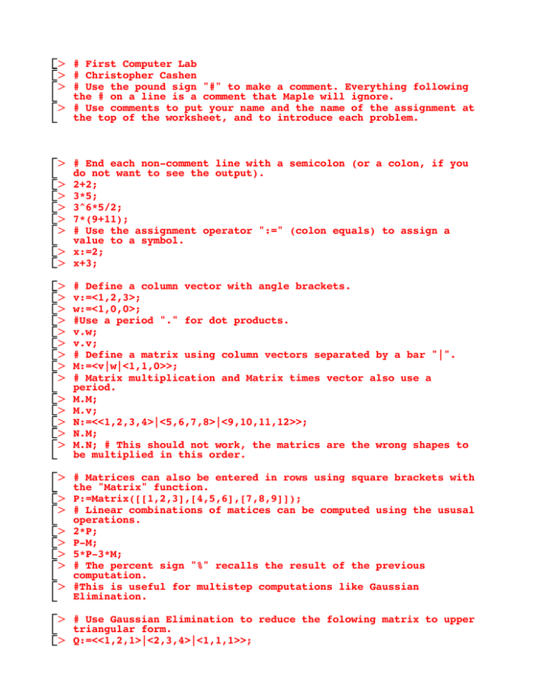
O # First Computer Lab
O # Christopher Cashen
O # Use the pound sign "#" to make a comment. Everything following
the # on a line is a comment that Maple will ignore.
O # Use comments to put your name and the name of the assignment at
the top of the worksheet, and to introduce each problem.
O # End each non-comment line with a semicolon (or a colon, if you
do not want to see the output).
O 2+2;
O 3*5;
O 3^6*5/2;
O 7*(9+11);
O # Use the assignment operator ":=" (colon equals) to assign a
value to a symbol.
O x:=2;
O x+3;
O
O
O
O
O
O
O
O
O
O
O
O
O
O
# Define a column vector with angle brackets.
v:=<1,2,3>;
w:=<1,0,0>;
#Use a period "." for dot products.
v.w;
v.v;
# Define a matrix using column vectors separated by a bar "|".
M:=<v|w|<1,1,0>>;
# Matrix multiplication and Matrix times vector also use a
period.
M.M;
M.v;
N:=<<1,2,3,4>|<5,6,7,8>|<9,10,11,12>>;
N.M;
M.N; # This should not work, the matrics are the wrong shapes to
be multiplied in this order.
O # Matrices can also be entered in rows using square brackets with
the "Matrix" function.
O P:=Matrix([[1,2,3],[4,5,6],[7,8,9]]);
O # Linear combinations of matices can be computed using the ususal
operations.
O 2*P;
O P-M;
O 5*P-3*M;
O # The percent sign "%" recalls the result of the previous
computation.
O #This is useful for multistep computations like Gaussian
Elimination.
O # Use Gaussian Elimination to reduce the folowing matrix to upper
triangular form.
O Q:=<<1,2,1>|<2,3,4>|<1,1,1>>;
O <<1,-2,-1>|<0,1,0>|<0,0,1>>.%;
O <<1,0,0>|<0,1,2>|<0,0,1>>.%;
O # You can use up to 3 percent signs at a time. %%% recalls the
result of the third to last computation.
O %%%;
O # Be careful using % because it recalls the last result in
memory, not the last result on the page. Try this example.
O 2+2;
O 4+3;
O # Use the mouse to move the cursor back up to the 2+2 line and
hit return to execute the computation. Then use the mouse ot move
the cursor to the line after this one.
O %;
O # The matrix Q has three non-zero pivots, so it is invertible.
You can ask for the inverse using two different notations. Let's
also check that the inverse times Q is the identity matrix.
O Q^(-1); 1/Q; %.Q;
O # We can also do symbolic computations.
O A:=Matrix([[a[1,1], a[1,2]],[a[2,1],a[2,2]]]);
O B:=Matrix([[b[1,1], b[1,2]],[b[2,1],b[2,2]]]);
O
O
O
O
O
O
O
O
O
O
O
O
O
O
O
O
O
O
C:=Matrix([[c[1,1], c[1,2]],[c[2,1],c[2,2]]]);
# Verify associativity of matrix multiplication.
(A.B).C-A.(B.C);
# That looks complicated, we expected to get the zero matrix.
Sometimes Maple needs a little encouragement to simplify
algebraic expressions.
simplify(%);
# It's good practice to do elimination step by step, but of
course we would like Maple to do it for us.
# To do this we need to load some additional functions using the
"with" command. Use a semicolon to see a list of all the
functions this gives us, or a colon to suppress the output.
with(LinearAlgebra):
Q;
GaussianElimination(Q);
# We can also do Gauss-Jordan Elimination using the function
"ReducedRowEchelonForm".
ReducedRowEchelonForm(Q);
# That's not very helpful; the reduced row echelon form of any
invertible matirx is the identity. However, the command also
works on augmented matrices.
R:=<Q|<1,2,3>>;
ReducedRowEchelonForm(R);
# There is also an interactive Gauss-Jordan Elimination Tutorial
available by including the Student[LinearAlgebra] package.
with(Student[LinearAlgebra]):
GaussJordanEliminationTutor(R);
O # You can generate random matrices to experiment with using the
RandomMatrix function.
O RandomMatrix(4);
O RandomMatrix(2,3);
O # Try Gauss-Jordan Elimination step by step on a random 3x4
matrix.