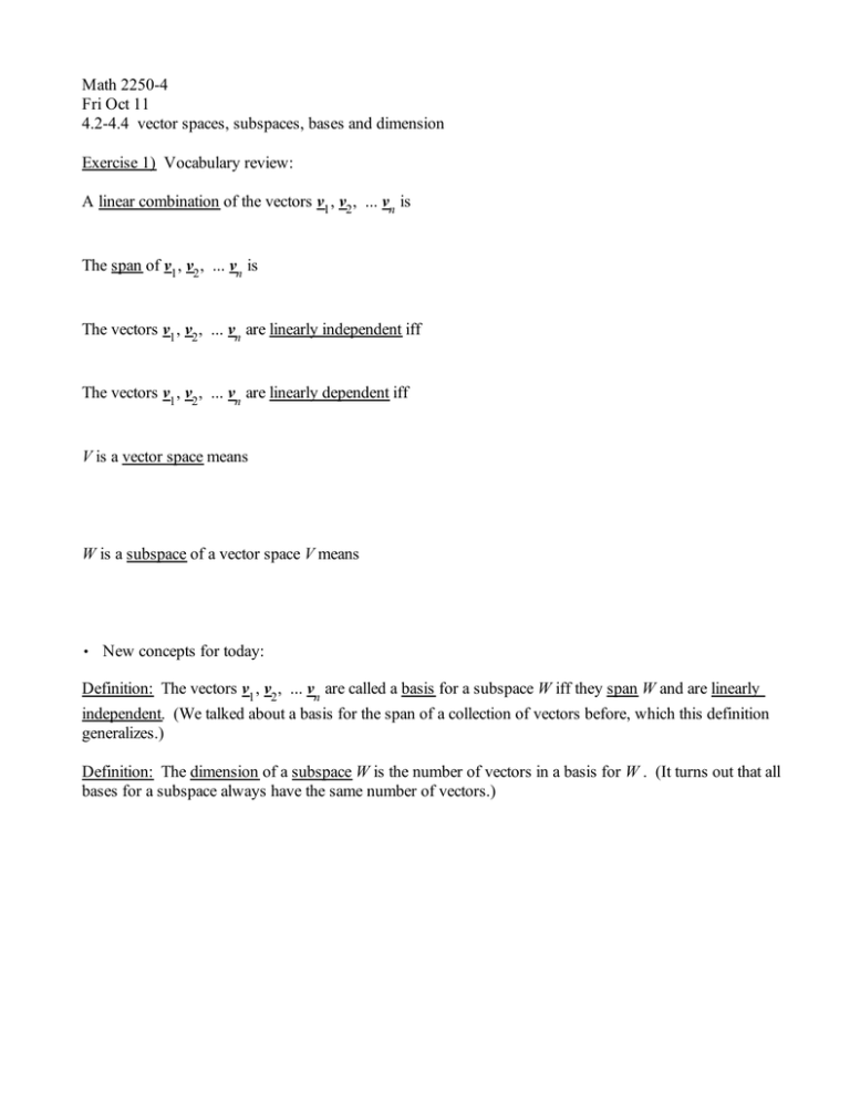
Math 2250-4
Fri Oct 11
4.2-4.4 vector spaces, subspaces, bases and dimension
Exercise 1) Vocabulary review:
A linear combination of the vectors v1 , v2 , ... vn is
The span of v1 , v2 , ... vn is
The vectors v1 , v2 , ... vn are linearly independent iff
The vectors v1 , v2 , ... vn are linearly dependent iff
V is a vector space means
W is a subspace of a vector space V means
, New concepts for today:
Definition: The vectors v1 , v2 , ... vn are called a basis for a subspace W iff they span W and are linearly
independent. (We talked about a basis for the span of a collection of vectors before, which this definition
generalizes.)
Definition: The dimension of a subspace W is the number of vectors in a basis for W . (It turns out that all
bases for a subspace always have the same number of vectors.)
As we've been seeing in examples, and will take care to understand today, there are two ways that
subspaces W arise naturally:
1) W is expressed as the span of a given collection v1 , v2 , ... vn of vectors. This is an explicit way to
describe W.
2) W is expressed as the collection of all solutions to some homogeneous matrix equation, i.e. the solution
space to a matrix equation A x = 0. This is an implicit way to describe W.
Often the subspace W is first expressed implicitly, and we would like an explicit description, ideally as the
span of a collection of basis vectors.
Theorem 1) The span of any collection of vectors v1 , v2 , ... vn in =m (or actually the span of any
f1 , f2 , ... fn in some vector space V) is closed under addition and scalar multiplication, and so is a subspace
of =m (or V .
why: We need to show W d span v1 , v2 , ... vn is a closed under addition and b closed under
scalar multiplication. Let
v = c1 v1 C c2 v2 C ...C cn vn 2 W
w = d1 w1 C d2 w2 C ...C dn wn 2 W
a
Then using the algebra properties of addition and scalar multiplication to rearrange and collect terms,
v C w = c1 C d1 v1 C c2 C d2 v2 C ...C cn C dn vn .
Thus v C w is also a linear combination of v1 , v2 , ... vn , so v C w 2 W is true.
b
Using algebra to rearrange terms we also compute
c v = cc1 v1 C cc2 v2 C ...C ccn vn 2 W
A
We will use Theorem 1 and matrix algebra to show that the geometry of subspaces in =m is pretty special:
Exercise 2) Use geometric reasoning to argue why the only subspaces of =2 are
(0) The single vector 0, 0 T , or
(1) A line through the origin, i.e. span u for some non-zero vector u , or
(2) All of =2 .
Exercise 3) Use matrix theory to show that the only subspaces of =3 are
(0) The single vector 0, 0, 0 T , or
(1) A line through the origin, i.e. span u for some non-zero vector u , or
(2) A plane through the origin, i.e.span u, v where u, v are linearly independent, or
(3) All of =3 .
Exercise 4) What are the dimensions of the subspaces in Exercise 2 and Exercise 3? How do the ideas in
Exercise 3 generalize to =n ?
Exercise 5) On Monday we showed that the plane in =3 explicity described as
1
K1
W d span
0 ,
2
2
0
has implicit equation
2 x C yKz = 0 .
In other words, an equivalent way to describe W would be implicitly, as
x
Wd
y s.t. 2 x C yKz = 0 .
z
Suppose you were just given the implicit equation. How could you find a basis for this plane if you didn't
have one already? (An example like this was actually one of your homework problems due today, and it
came with a hint that we will utilize.)
This example leads to
Theorem 2: Let Am # n be a matrix. Consider the solution space W of all solutions to the homogeneous
matrix equation
Ax=0 ,
i.e.
W = x 2 =n s.t. Am # n x = 0 .
Then W 4 =n is a subspace. Furthermore, you can find a basis for this subspace by backsolving from the
reduced row echelon form of A: once you write the solution in linear combination form
x = c1 v1 C c2 v2 C ...C ck vk
the vectors v1 , v2 , ... vk will always be linearly independent. Thus, since these vectors span W by
construction, v1 , v2 , ... vk are a basis for W.
Exercise 6) Check from the implicit description that a , b hold for the solution space W to A x = 0 ,
i.e to verify that
W = x 2 =n s.t. Am # n x = 0
is indeed a subspace (without using the fact that we can write the solution space explicitly as the span of
some vectors). This problem is akin to some of the postponed homework problems from section 4.2.
Illustrate how to find a basis for the solution space to a homogeneous matrix equation by completing this
large example:
Exercise 7) Consider the matrix equation A x = 0 , with the matrix A (and its reduced row echelon form)
shown below:
1 2 0 1 1 2
1 2 0 1 1 2
A :=
2
4 1
K1 K2 1
4
1
7
1 K2
1
/
0 0 1 2 K1 3
0 0 0 0
0 0
K2 K4 0 K2 K2 K4
0 0 0 0 0 0
7a) Find a basis for the solution space W = x 2 =6 s.t. A x = 0 by backsolving, writing your explicit
solutions in linear combination form, and extracting a basis. Explain why these vectors span the solution
space and verify that they're linearly independent.
7b) What is the dimension of W ? How is the dimension related to the shape of the reduced row echelon
form of A?
Exercise 8) Focus on the idea that solutions to homogeneous matrix equations correspond exactly to linear
dependencies between the columns of the matrix. (If it helps, think of renaming the vector x in the example
above, with a vector c of linear combination coefficients.) Since the solution set to a homogeneous linear
system does not change as you do elementary row operations to the augmented matrix, column
dependencies also do not change. Therfore your basis in 7a for the homogeneous solution space can also
be thought of as a "basis" of the key column dependencies, for both the original matrix, and for the
reduced row echelon form. Check this, by reading off "easy" column dependencies in the reduced matrix,
and seeing that they are also dependencies in the original matrix (and that they correspond to the basis of
the homogeneous solution space). Magic! One can use this magic in interesting ways, as we will see
later.
Remark: This "magic" connection via the homogeneous solutions space, guaranteeing that column
dependencies are the same in a matrix and in its reduced row echelon form explains the mystery of why
each matrix has only one reduced row echelon form, no matter which sequence of elementary row
operations one uses to compute it: The four conditions for rref (zero rows at bottom, non-zero rows start
with leading ones, leading ones in successive rows move to the right, all column entries in any column
containing a leading "1" are zero except for that "1"), together with the column dependencies of the original
(and hence reduced matrix) uniquely determine the rref matrix. Check with the example in Exercise 7!