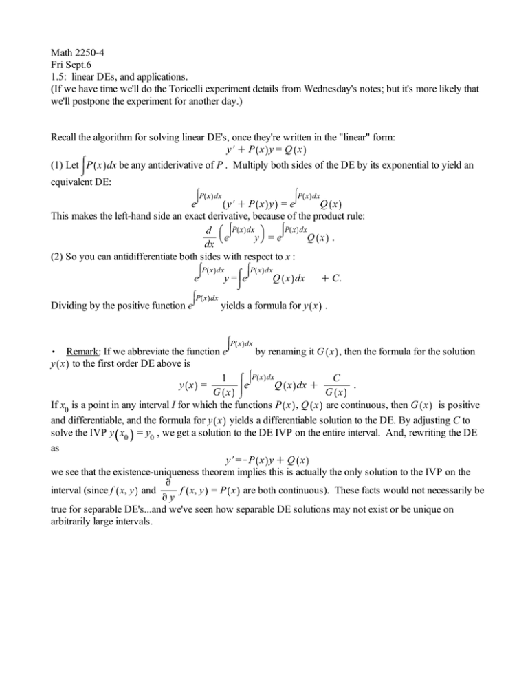
Math 2250-4
Fri Sept.6
1.5: linear DEs, and applications.
(If we have time we'll do the Toricelli experiment details from Wednesday's notes; but it's more likely that
we'll postpone the experiment for another day.)
Recall the algorithm for solving linear DE's, once they're written in the "linear" form:
y#C P x y = Q x
(1) Let P x dx be any antiderivative of P . Multiply both sides of the DE by its exponential to yield an
equivalent DE:
P x dx
P x dx
e
y#C P x y = e
Q x
This makes the left-hand side an exact derivative, because of the product rule:
P x dx
P x dx
d
e
y =e
Q x .
dx
(2) So you can antidifferentiate both sides with respect to x :
e
Dividing by the positive function e
P x dx
P x dx
y= e
P x dx
Q x dx
C C.
yields a formula for y x .
P x dx
, Remark: If we abbreviate the function e
by renaming it G x , then the formula for the solution
y x to the first order DE above is
P x dx
1
C
y x =
e
Q x dx C
.
G x
G x
If x0 is a point in any interval I for which the functions P x , Q x are continuous, then G x is positive
and differentiable, and the formula for y x yields a differentiable solution to the DE. By adjusting C to
solve the IVP y x0 = y0 , we get a solution to the DE IVP on the entire interval. And, rewriting the DE
as
y#=KP x y C Q x
we see that the existence-uniqueness theorem implies this is actually the only solution to the IVP on the
v
interval (since f x, y and
f x, y = P x are both continuous). These facts would not necessarily be
vy
true for separable DE's...and we've seen how separable DE solutions may not exist or be unique on
arbitrarily large intervals.
Exercise 1: Find all solutions to the linear (and separable) DE
6 xK3 x y
y# x =
x2 C 1
Hint: as you can verify below, the general solution is y x = 2 C C x2 C 1
> with DEtools :
dsolve
3
2
K
.
An extremely important class of modeling problems that lead to linear DE's involve input-output models.
These have diverse applications ranging from bioengineering to environmental science. For example, The
"tank" below could actually be a human body, a lake, or a pollution basin, in different applications.
For the present considerations, consider a tank holding liquid, with volume V t (e.g units l ). Liquid
l
gm
flows in at a rate ri (e.g. units
), and with solute concentration ci (e.g. units
). Liquid flows out at a
s
l
rate ro , and with concentration c0 . We are attempting to model the volume V t of liquid and the amount
of solute x t (e.g. units gm ) in the tank at time t , given V 0 = V0 , x 0 = x0 . We assume the solution
in the tank is well-mixed, so that we can treat the concentration as uniform throughout the tank, i.e.
x t
gm
co =
.
V t
l
See the diagram below.
Exercise 2: Under these assumptions use your modeling ability and Calculus to derive the following
differential equations for V t and x t :
a) The DE for V t , which we can just integrate:
V# t = ri K r0
t
so V t = V0 C
0
ri t K r0 t dt
b) The linear DE for x t .
x# t = ri ci K ro co = ri ci Kro
x# t C
ro
V
x t = ri ci
x
V
Often (but not always) the tank volume remains constant, i.e. ri = ro . If the incoming concentration ci is
also constant, then the IVP for solute amount is
x#C a x = b
x 0 = x0
where a, b are constants.
Exercise 3: The constant coefficient initial value problem above will recur throughout the course in various
contexts, so let's solve it now. Hint: We will check our answer with Maple first, and see that the solution
is
b
b Ka t
x t =
C xo K
e
.
a
a
Exercise 4: Use the result above to solve a pollution problem IVP and answer the following question (p.
55-56 text): Lake Huron has a pretty constant concentration for a certain pollutant. Due to an industrial
accident, Lake Erie has suddenly obtained a concentration five times as large. Lake Erie has a volume of
480 km3 , and water flows into and out of Lake Erie at a rate of 350 km3 per year. Essentially all of the inflow is from Lake Huron (see below). We expect that as time goes by, the water from Lake Huron will
flush out Lake Erie. Assuming that the pollutant concentration is roughly the same everywhere in Lake
Erie, about how long will it be until this concentration is only twice the background concentration from
Lake Huron?
http://www.enchantedlearning.com/usa/statesbw/greatlakesbw.GIF
a) Set up the initial value problem. Maybe use symbols
c for the background concentration (in Huron),
V = 480 km3
km3
r = 350
y
b) Solve the IVP, and then answer the question.