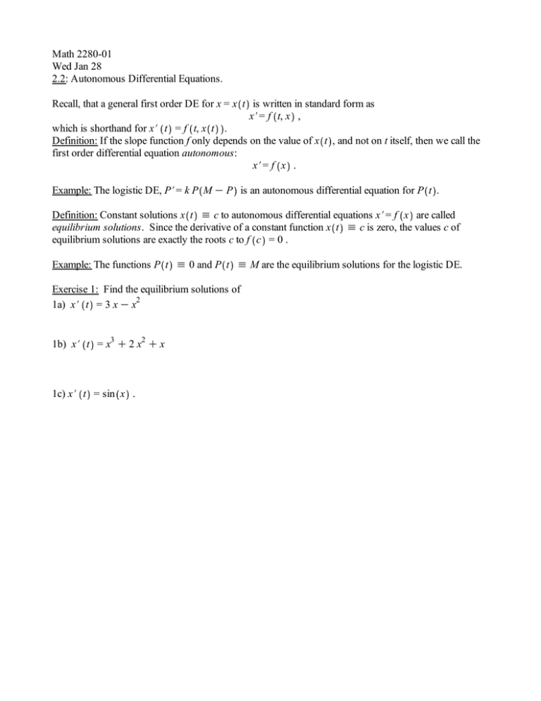
Math 2280-01
Wed Jan 28
2.2: Autonomous Differential Equations.
Recall, that a general first order DE for x = x t is written in standard form as
x#= f t, x ,
which is shorthand for x# t = f t, x t .
Definition: If the slope function f only depends on the value of x t , and not on t itself, then we call the
first order differential equation autonomous:
x#= f x .
Example: The logistic DE, P#= k P M K P is an autonomous differential equation for P t .
Definition: Constant solutions x t h c to autonomous differential equations x#= f x are called
equilibrium solutions. Since the derivative of a constant function x t h c is zero, the values c of
equilibrium solutions are exactly the roots c to f c = 0 .
Example: The functions P t h 0 and P t h M are the equilibrium solutions for the logistic DE.
Exercise 1: Find the equilibrium solutions of
1a) x# t = 3 x K x2
1b) x# t = x3 C 2 x2 C x
1c) x# t = sin x .
Def: Let x t h c be an equilibrium solution for an autonomous DE. Then
· c is a stable equilibrium solution if solutions with initial values close enough to c stay close to c.
There is a precise way to say this, but it requires quantifiers: For every e O 0 there exists a d O 0 so that
for solutions with x 0 K c ! d, we have x t K c ! e for all t O 0 .
· c is an unstable equilibrium if it is not stable.
· c is an asymptotically stable equilibrium solution if it's stable and in addition, if x 0 is close enough
to c , then t lim
x t = c, i.e. there exists a d O 0 so that if x 0 K c ! d then
/N
lim x t = c . (Notice that this means the horizontal line x = c will be an asymptote to the solution graphs
t /N
x = x t in these cases.)
Exercise 2: Use phase diagram analysis to guess the stability of the equilibrium solutions in Exercise 1.
For (a) you've worked out a solution formula already, so you'll know you're right. For (b), (c), use the
Theorem on the next page to justify your answers.
2a) x# t = 3 x K x2
2b) x# t = x3 C 2 x2 C x
2c) x# t = sin x .
Theorem: Consider the autonomous differential equation
x# t = f x
v
with f x and
f x continuous (so local existence and uniqueness theorems hold). Let f c = 0 , i.e.
vx
x t h c is an equilibrium solution. Suppose c is an isolated zero of f, i.e. there is an open interval
containing c so that c is the only zero of f in that interval. The the stability of the equilibrium solution c can
is completely determined by the local phase diagrams:
sign f : KKKK0 CCC
0 )))c/// 0 c is unstable
sign f : CCC 0 KKKK 0 ///c))) 0 c is asymptotically stable
sign f : CCC 0 CCC 0 ///c/// 0 c is unstable (half stable)
sign f :KKKK0 KKKK 0 )))c))) 0 c is unstable (half stable)
You can actually prove this Theorem with calculus!! (want to try?)
Here's why!
Exercise 3) Use the chain rule to check that if x t solves the autonomous DE
x# t = f x
Then X t d x t K c solves the same DE. What does this say about the geometry of representative
solution graphs to autonomous DEs? Have we already noticed this?
Further application: Doomsday-extinction. With different hypotheses about fertility and mortality rates,
one can arrive at a population model which looks like logistic, except the right hand side is the opposite of
what it was in that case:
Logistic:
P# t =Ka P2 C b P
Doomsday-extinction: Q # t = a Q2 K b Q
For example, suppose that the chances of procreation are proportional to population density (think
alligators or crickets), i.e. the fertility rate b = a Q t , where Q t is the population at time t. Suppose the
morbidity rate is constant, d = b. With these assumptions the birth and death rates are a Q2 and Kb Q ....
which yields the DE above. In this case factor the right side:
b
Q# t = a Q Q K
= k Q QKM .
a
Exercise 4a) Construct the phase diagram for the general doomsday-extinction model and discuss the
stability of the equilbrium solutions.
Exercise 4b) If P t solves the logistic differential equation
P# t = k P M K P
show that Q t d P Kt solves the doomsday-extinction differential equation
Q# t = k Q Q K M .
Use this to recover a formula for solutions to doomsday-extinction IVPs. What does this say about how
representative solution graphs are related, for the logistic and the doomsday-extinction models? Recall, the
solution to the logistic IVP is
MP0
P t =
.
M K P0 eKMkt C P0
Exercise 5: Use your formula from the previous exercise or work the separable DE from scratch, to
transcribe the solution to the doomsday-extinction IVP
x# t = x x K 1
x 0 =2.
Does the solution exist for all t O 0 ? (Hint: no, there is a very bad doomsday at t = ln 2.