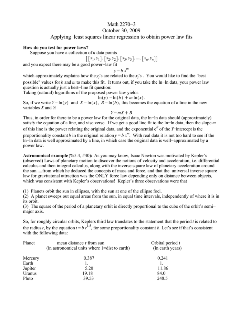
Math 2270−3
October 30, 2009
Applying least squares linear regression to obtain power law fits
How do you test for power laws?
Suppose you have a collection of n data points
x1, y1 , x2, y2 , x3, y3 , ..., xn, yn
and you expect there may be a good power−law fit
y = b xm
which approximately explains how the yi’s are related to the xi’s . You would like to find the "best
possible" values for b and m to make this fit. It turns out, if you take the ln−ln data, your power law
question is actually just a best−line fit question:
Taking (natural) logarithms of the proposed power law yields
ln y = ln b
m ln x .
So, if we write Y = ln y and X = ln x , B = ln b , this becomes the equation of a line in the new
variables X and Y:
Y = mX B
Thus, in order for there to be a power law for the original data, the ln−ln data should (approximately)
satisfy the equation of a line, and vise verse. If we get a good line fit to the ln−ln data, then the slope m
of this line is the power relating the original data, and the exponential eB of the Y−intercept is the
proportionality constant b in the original relation y = b xm. With real data it is not too hard to see if the
ln−ln data is well approximated by a line, in which case the original data is well−approximated by a
power law.
Astronomical example (%5.4, #40): As you may know, Isaac Newton was motivated by Kepler’s
(observed) Laws of planetary motion to discover the notions of velocity and acceleration, i.e. differential
calculus and then integral calculus, along with the inverse square law of planetary acceleration around
the sun.....from which he deduced the concepts of mass and force, and that the universal inverse square
law for gravitatonal attraction was the ONLY force law depending only on distance between objects,
which was consistent with Kepler’s observations! Kepler’s three observations were that
(1) Planets orbit the sun in ellipses, with the sun at one of the ellipse foci.
(2) A planet sweeps out equal areas from the sun, in equal time intervals, independently of where it is in
its orbit.
(3) The square of the period of a planetary orbit is directly proportional to the cube of the orbit’s semi−
major axis.
So, for roughly circular orbits, Keplers third law translates to the statement that the period t is related to
the radius r, by the equation t = b r1.5, for some proportionality constant b. Let’s see if that’s consistent
with the following data:
Planet
Mercury
Earth
Jupiter
Uranus
Pluto
mean distance r from sun
(in astronomical units where 1=dist to earth)
0.387
1.
5.20
19.18
39.53
Orbital period t
(in earth years)
0.241
1.
11.86
84.0
248.5
Maple implementation:
with LinearAlgebra : #LinearAlgebra command package
with plots : #plotting package
rs
Vector 0.387, 1., 5.20, 19.18, 39.53 : #radii
ts
Vector .241, 1., 11.86, 84.0, 248.5 : #corresponding periods
pts
seq rs i , ts i , i = 1 ..5 : #points in the r−t plane
Rs
Ts
Rs
Ts
lnpts
lnpts
ones
A
map ln, rs : #logs of radii
map ln, ts : #logs of periods
map evalf, Rs : #compute decimal values − don’t forget this step for your BMI work!
map evalf, Ts :
seq Rs i , Ts i , i = 1 ..5 : #points in the lnr−lnt plane
Rs Ts : # a better way! (thanks Jim S.)
Vector 1, 1, 1, 1, 1 : #a column for the linear regression fit matrix
Rs ones ;
0.9493305860 1
A :=
0.
1
1.648658626
1
2.953868069
1
3.677059877
1
AT
Transpose A :
AT.A 1. AT.Ts ; #least squares solution, m, ln b !
#notice, our data agrees with Kepler!
1.49981641316970692
0.000486890692341201970
b
exp 0.000486890692341201970 : #recover proportionality constant
(1)
(2)
lnplot1
plot 1.49982 R .0004860, R = 1 ..4, T = 2 ..6, color = black :
#linear regression line for lnr−lnt data
lnplot2
pointplot lnpts, color = red : #actual ln−ln data
display lnplot1, lnplot2 , title = ‘ln−ln line fit‘ ;
ln−ln line fit
6
5
4
T
3
2
1
1
1
1
2
R
3
4
2
plot1
plot b r1.4998, r = 0 ..40, t = 0 ..250, color = black : #almost Kepler power law
plot2
pointplot pts, color = red : #radius−period points for planets
display plot1, plot2 , title = ‘Kepler and Newton were right‘ ;
Kepler and Newton were right
250
200
150
t
100
50
0
0
10
20
r
30
40