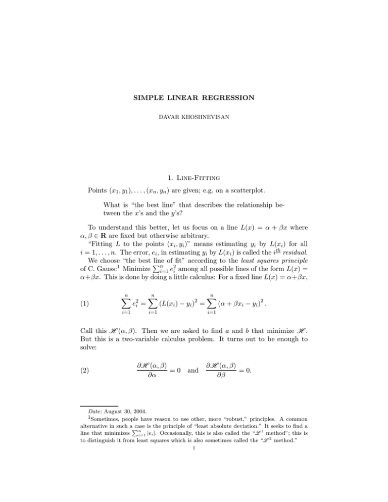
SIMPLE LINEAR REGRESSION
DAVAR KHOSHNEVISAN
1. Line-Fitting
Points (x1 , y1 ), . . . , (xn , yn ) are given; e.g. on a scatterplot.
What is “the best line” that describes the relationship between the x’s and the y’s?
To understand this better, let us focus on a line L(x) = α + βx where
α, β ∈ R are fixed but otherwise arbitrary.
“Fitting L to the points (xi , yi )” means estimating yi by L(xi ) for all
i = 1, . . . , n. The error, ei , in estimating yi by L(xi ) is called the ith residual.
We choose “the best P
line of fit” according to the least squares principle
of C. Gauss:1 Minimize ni=1 e2i among all possible lines of the form L(x) =
α+βx. This is done by doing a little calculus: For a fixed line L(x) = α+βx,
n
X
(1)
i=1
e2i =
n
X
(L(xi ) − yi )2 =
i=1
n
X
(α + βxi − yi )2 .
i=1
H
H
Call this
(α, β). Then we are asked to find a and b that minimize
.
But this is a two-variable calculus problem. It turns out to be enough to
solve:
(2)
∂
H (α, β) = 0
∂α
and
∂
H (α, β) = 0.
∂β
Date: August 30, 2004.
1Sometimes, people have reason to use other, more “robust,” principles. A common
alternative in such aP
case is the principle of “least absolute deviation.” It seeks to find a
1
line that minimizes n
method”; this is
i=1 |ei |. Occasionally, this is also called the “
to distinguish it from least squares which is also sometimes called the “ 2 method.”
L
1
L
2
DAVAR KHOSHNEVISAN
First,
∂
H (α, β) = X 2(α + βx − y )
n
∂α
i
i=1
= 2αn + 2β
(3)
∂
n
X
i
xi − 2
i=1
n
X
H (α, β) = X 2(α + βx − y )x
n
∂β
i
i=1
= 2α
n
X
xi + 2β
i=1
yi , and
i=1
i
n
X
i=1
i
x2i − 2
n
X
xi y i .
i=1
These are called the normal equations. Now (2) is transformed into two
equations in two unknowns [α and β]:
(4)
αx + βx2 = xy
α + βx = y.
Multiply the second equation of (4) by x, and then subtract from the
first equation to find that β(x2 − (x)2 ) = xy − x · y. You should recognize this, in statistical terms, as βVar(x) = Cov(x, y). Equivalently,
β = Cov(x, y)/Var(x) = Corr(x, y)SDy /SDx . Plug this into the second equation of (4) to find that α = y − βx for the computed β. To summarize,
Theorem 1.1. The least-squares line through (x1 , y1 ), . . . , (xn , yn ) is unique
and defined by
b − x), where βb = Corr(x, y) SDy .
(5)
L(x) = y + β(x
SDx
2. The Measurement-Error Model
Let Y = (Y1 , . . . , Yn ) be a random sample of n i.i.d. copies of the response
variable. The measurement-error model posits the following:
(6)
Yi = α + βXi + εi
i = 1, . . . , n.
Here, X = (X1 , . . . , Xn ) is a non-random vector of constants—the explanatory variables—and α and β are unknown parameters. This model also
assumes that the εi ’s are i.i.d. N (0, σ 2 ) for an unknown parameter σ > 0.
The Yi ’s are random only because the εi ’s are (and not the Xi ’s).
According to the principle of least squares (Theorem 1.1), the best leastsquares estimates of α and β are, respectively,
1 Pn
i=1 Xi Yi − X · Y
n
b
(7)
β= 1P
and α
b =Y −α
bX.
n
2
i=1 (Xi − X)
n
The more imortant parameter is β. For instance, consider the test,
(8)
H0 : β = 0
vs. H1 : β 6= 0.
SIMPLE LINEAR REGRESSION
3
This is testing the hypothesis that the explanatory variable X has a (linear)
effect on Y .
b Note that
So we need the distribution of β.
Pn
n
X
i=1 Yi Xi − X
b
β = Pn
=
bi Y i ,
(9)
2
i=1 (Xi − X)
i=1
where
(10)
Xi − X
bi =
ns2X
for
s2X
n
1X
=
(Xi − X)2 .
n
i=1
Recall that the Xi ’s are not random. Therefore, neither are the bi ’s. Also
recall,
Lemma 2.1. If V1 , . . . ,P
Vn are independent and Vi ∼ N (µi , σi2 ), then for all
non-random c1 , . . . , cn , ni=1 ci Vi ∼ N (µ, σ 2 ) where µ = µ1 + · · · + µn and
σ 2 = σ12 + · · · + σ22 .
P
P
Consequently, βb ∼ N ( ni=1 bi E[Yi ], ni=1 b2i Var(Yi )). But Yi = α + βXi +
2
εi . So, E[Y
and Var(Yi ) = Var(εi ) =
is easy to check
Pni ] = α + βXi , P
Pσn . It
n
that: (i) i=1 bi = 0; (ii) i=1 bi Xi = 1; and (iii) i=1 b2i = 1/(ns2X ). This
proves that
2
σ
(11)
βb ∼ N β, 2 .
nsX
b = β. That is, βb is an unbiased estimator of β. Moreover,
Therefore, E[β]
2
if we knew σ , then we could perform the test of hypothesis (8) at any
predescribed level, say at 95%. The trouble is that we generally do not
know σ 2 .
P
Because the Yi ’s have variance σ 2 , we can estimate σ 2 by s2Y = n1 ni=1 (Yi −
b s2 ). The key to this
Y )2 . But then we need the joint distribution of (β,
Y
theory is that βb is independent of s2Y . We just determined the distribution
b and we will see later on that the H0 -distribution of s2 is essentially
of β,
Y
2
χ . The rest will be smooth sailing.
To recap, we need to accomplish two things:
(1) Derive the independence of βb and s2Y ; and
(2) Honestly compute the distribution of s2Y under H0 .
Just about all of this semester’s work is concerned with accomplishing these
two goals (for more general models).